备注
Click here to download the full example code
架构搜索入门教程
这是 NNI 上的神经架构搜索(NAS)的入门教程。 在本教程中,我们将借助 NNI 的 NAS 框架,即 Retiarii,在 MNIST 数据集上实现网络结构搜索。 我们以多尝试的架构搜索为例来展示如何构建和探索模型空间。
神经架构搜索任务主要有三个关键组成部分,即
模型搜索空间,定义了一个要探索的模型的集合。
一个合适的策略作为探索这个模型空间的方法。
一个模型评估器,用于为搜索空间中每个模型评估性能。
目前,Retiarii 只支持 PyTorch,并对 PyTorch 1.7 到 1.10 进行了测试。 所以本教程假定您使用 PyTorch 作为深度学习框架。未来我们会支持更多框架。
定义您的模型空间
模型空间是由用户定义的,用来表达用户想要探索的一组模型,其中包含有潜力的好模型。 在 NNI 的框架中,模型空间由两部分定义:基本模型和基本模型上可能的变化。
定义基本模型
定义基本模型与定义 PyTorch(或 TensorFlow)模型几乎相同。
通常,您只需将代码 import torch.nn as nn 替换为
import nni.retiarii.nn.pytorch as nn 以使用我们打包的 PyTorch 模块。
下面是定义基本模型的一个非常简单的示例。
import torch
import torch.nn.functional as F
import nni.retiarii.nn.pytorch as nn
from nni.retiarii import model_wrapper


@model_wrapper      # this decorator should be put on the out most
class Net(nn.Module):
    def __init__(self):
        super().__init__()
        self.conv1 = nn.Conv2d(1, 32, 3, 1)
        self.conv2 = nn.Conv2d(32, 64, 3, 1)
        self.dropout1 = nn.Dropout(0.25)
        self.dropout2 = nn.Dropout(0.5)
        self.fc1 = nn.Linear(9216, 128)
        self.fc2 = nn.Linear(128, 10)

    def forward(self, x):
        x = F.relu(self.conv1(x))
        x = F.max_pool2d(self.conv2(x), 2)
        x = torch.flatten(self.dropout1(x), 1)
        x = self.fc2(self.dropout2(F.relu(self.fc1(x))))
        output = F.log_softmax(x, dim=1)
        return output
小技巧
记住,您应该使用 import nni.retiarii.nn.pytorch as nn 和 nni.retiarii.model_wrapper()。
许多错误都是因为忘记使用某一个。
另外,要使用 nn.init 的子模块,可以使用 torch.nn,例如, torch.nn.init 而不是 nn.init。
定义模型变化
基本模型只是一个具体模型,而不是模型空间。 我们提供 模型变化的 API 让用户表达如何改变基本模型。 即构建一个包含许多模型的搜索空间。
基于上述基本模型,我们可以定义如下模型空间。
@model_wrapper
class Net(nn.Module):
  def __init__(self):
    super().__init__()
    self.conv1 = nn.Conv2d(1, 32, 3, 1)
-   self.conv2 = nn.Conv2d(32, 64, 3, 1)
+   self.conv2 = nn.LayerChoice([
+       nn.Conv2d(32, 64, 3, 1),
+       DepthwiseSeparableConv(32, 64)
+   ])
-   self.dropout1 = nn.Dropout(0.25)
+   self.dropout1 = nn.Dropout(nn.ValueChoice([0.25, 0.5, 0.75]))
    self.dropout2 = nn.Dropout(0.5)
-   self.fc1 = nn.Linear(9216, 128)
-   self.fc2 = nn.Linear(128, 10)
+   feature = nn.ValueChoice([64, 128, 256])
+   self.fc1 = nn.Linear(9216, feature)
+   self.fc2 = nn.Linear(feature, 10)

  def forward(self, x):
    x = F.relu(self.conv1(x))
    x = F.max_pool2d(self.conv2(x), 2)
    x = torch.flatten(self.dropout1(x), 1)
    x = self.fc2(self.dropout2(F.relu(self.fc1(x))))
    output = F.log_softmax(x, dim=1)
    return output
结果是以下代码:
class DepthwiseSeparableConv(nn.Module):
    def __init__(self, in_ch, out_ch):
        super().__init__()
        self.depthwise = nn.Conv2d(in_ch, in_ch, kernel_size=3, groups=in_ch)
        self.pointwise = nn.Conv2d(in_ch, out_ch, kernel_size=1)

    def forward(self, x):
        return self.pointwise(self.depthwise(x))


@model_wrapper
class ModelSpace(nn.Module):
    def __init__(self):
        super().__init__()
        self.conv1 = nn.Conv2d(1, 32, 3, 1)
        # LayerChoice is used to select a layer between Conv2d and DwConv.
        self.conv2 = nn.LayerChoice([
            nn.Conv2d(32, 64, 3, 1),
            DepthwiseSeparableConv(32, 64)
        ])
        # ValueChoice is used to select a dropout rate.
        # ValueChoice can be used as parameter of modules wrapped in `nni.retiarii.nn.pytorch`
        # or customized modules wrapped with `@basic_unit`.
        self.dropout1 = nn.Dropout(nn.ValueChoice([0.25, 0.5, 0.75]))  # choose dropout rate from 0.25, 0.5 and 0.75
        self.dropout2 = nn.Dropout(0.5)
        feature = nn.ValueChoice([64, 128, 256])
        self.fc1 = nn.Linear(9216, feature)
        self.fc2 = nn.Linear(feature, 10)

    def forward(self, x):
        x = F.relu(self.conv1(x))
        x = F.max_pool2d(self.conv2(x), 2)
        x = torch.flatten(self.dropout1(x), 1)
        x = self.fc2(self.dropout2(F.relu(self.fc1(x))))
        output = F.log_softmax(x, dim=1)
        return output


model_space = ModelSpace()
model_space
Out:
ModelSpace(
  (conv1): Conv2d(1, 32, kernel_size=(3, 3), stride=(1, 1))
  (conv2): LayerChoice([Conv2d(32, 64, kernel_size=(3, 3), stride=(1, 1)), DepthwiseSeparableConv(
    (depthwise): Conv2d(32, 32, kernel_size=(3, 3), stride=(1, 1), groups=32)
    (pointwise): Conv2d(32, 64, kernel_size=(1, 1), stride=(1, 1))
  )], label='model_1')
  (dropout1): Dropout(p=0.25, inplace=False)
  (dropout2): Dropout(p=0.5, inplace=False)
  (fc1): Linear(in_features=9216, out_features=64, bias=True)
  (fc2): Linear(in_features=64, out_features=10, bias=True)
)
这个例子使用了两个模型变化的 API, nn.LayerChoice 和 nn.InputChoice。
nn.LayerChoice 可以从一系列的候选子模块中(在本例中为两个),为每个采样模型选择一个。
它可以像原来的 PyTorch 子模块一样使用。
nn.InputChoice 的参数是一个候选值列表,语义是为每个采样模型选择一个值。
更详细的 API 描述和用法可以在 这里 找到。
备注
我们正在积极丰富模型变化的 API,使得您可以轻松构建模型空间。 如果当前支持的模型变化的 API 不能表达您的模型空间, 请参考 这篇文档 来自定义突变。
探索定义的模型空间
简单来讲,有两种探索方法: (1) 独立评估每个采样到的模型,这是 多尝试 NAS 中的搜索方法。 (2) 单尝试共享权重型的搜索,简称单尝试 NAS。 我们在本教程中演示了第一种方法。第二种方法用户可以参考 这里。
首先,用户需要选择合适的探索策略来探索定义好的模型空间。 其次,用户需要选择或自定义模型性能评估来评估每个探索模型的性能。
选择探索策略
Retiarii 支持许多 探索策略。
只需选择(即实例化)探索策略,就如下面的代码演示的一样:
import nni.retiarii.strategy as strategy
search_strategy = strategy.Random(dedup=True)  # dedup=False if deduplication is not wanted
Out:
/home/yugzhan/miniconda3/envs/cu102/lib/python3.8/site-packages/ray/autoscaler/_private/cli_logger.py:57: FutureWarning: Not all Ray CLI dependencies were found. In Ray 1.4+, the Ray CLI, autoscaler, and dashboard will only be usable via `pip install 'ray[default]'`. Please update your install command.
  warnings.warn(
挑选或自定义模型评估器
在探索过程中,探索策略反复生成新模型。模型评估器负责训练并验证每个生成的模型以获得模型的性能。 该性能作为模型的得分被发送到探索策略以帮助其生成更好的模型。
Retiarii 提供了 内置模型评估器,但在此之前,
我们建议使用 FunctionalEvaluator,即用一个函数包装您自己的训练和评估代码。
这个函数应该接收一个单一的模型类并使用 nni.report_final_result() 报告这个模型的最终分数。
此处的示例创建了一个简单的评估器,该评估器在 MNIST 数据集上运行,训练 2 个 epoch,并报告其在验证集上的准确率。
import nni

from torchvision import transforms
from torchvision.datasets import MNIST
from torch.utils.data import DataLoader


def train_epoch(model, device, train_loader, optimizer, epoch):
    loss_fn = torch.nn.CrossEntropyLoss()
    model.train()
    for batch_idx, (data, target) in enumerate(train_loader):
        data, target = data.to(device), target.to(device)
        optimizer.zero_grad()
        output = model(data)
        loss = loss_fn(output, target)
        loss.backward()
        optimizer.step()
        if batch_idx % 10 == 0:
            print('Train Epoch: {} [{}/{} ({:.0f}%)]\tLoss: {:.6f}'.format(
                epoch, batch_idx * len(data), len(train_loader.dataset),
                100. * batch_idx / len(train_loader), loss.item()))


def test_epoch(model, device, test_loader):
    model.eval()
    test_loss = 0
    correct = 0
    with torch.no_grad():
        for data, target in test_loader:
            data, target = data.to(device), target.to(device)
            output = model(data)
            pred = output.argmax(dim=1, keepdim=True)
            correct += pred.eq(target.view_as(pred)).sum().item()

    test_loss /= len(test_loader.dataset)
    accuracy = 100. * correct / len(test_loader.dataset)

    print('\nTest set: Accuracy: {}/{} ({:.0f}%)\n'.format(
          correct, len(test_loader.dataset), accuracy))

    return accuracy


def evaluate_model(model_cls):
    # "model_cls" is a class, need to instantiate
    model = model_cls()

    device = torch.device('cuda') if torch.cuda.is_available() else torch.device('cpu')
    model.to(device)

    optimizer = torch.optim.Adam(model.parameters(), lr=1e-3)
    transf = transforms.Compose([transforms.ToTensor(), transforms.Normalize((0.1307,), (0.3081,))])
    train_loader = DataLoader(MNIST('data/mnist', download=True, transform=transf), batch_size=64, shuffle=True)
    test_loader = DataLoader(MNIST('data/mnist', download=True, train=False, transform=transf), batch_size=64)

    for epoch in range(3):
        # train the model for one epoch
        train_epoch(model, device, train_loader, optimizer, epoch)
        # test the model for one epoch
        accuracy = test_epoch(model, device, test_loader)
        # call report intermediate result. Result can be float or dict
        nni.report_intermediate_result(accuracy)

    # report final test result
    nni.report_final_result(accuracy)
创建评估器
from nni.retiarii.evaluator import FunctionalEvaluator
evaluator = FunctionalEvaluator(evaluate_model)
这里的 train_epoch 和 test_epoch 可以是任何自定义函数,用户可以在其中编写自己的训练逻辑。
建议这里的 evaluate_model 不接受除 model_cls 之外的其他参数。
但是,在 高级教程 </nas/evaluator> 中,我们将展示如何使用其他参数,以免您确实需要这些参数。
未来,我们将支持对评估器的参数进行变化(通常称为“超参数调优”)。
启动实验
一切都已准备就绪,现在就可以开始做模型搜索的实验了。如下所示。
from nni.retiarii.experiment.pytorch import RetiariiExperiment, RetiariiExeConfig
exp = RetiariiExperiment(model_space, evaluator, [], search_strategy)
exp_config = RetiariiExeConfig('local')
exp_config.experiment_name = 'mnist_search'
以下配置可以用于控制最多/同时运行多少试验。
exp_config.max_trial_number = 4   # 最多运行 4 个实验
exp_config.trial_concurrency = 2  # 最多同时运行 2 个试验
如果要使用 GPU,请设置以下配置。
如果您希望使用被占用了的 GPU(比如 GPU 上可能正在运行 GUI),则 use_active_gpu 应设置为 true。
exp_config.trial_gpu_number = 1
exp_config.training_service.use_active_gpu = True
启动实验。 在一个有两块 GPU 的工作站上完成整个实验大约需要几分钟时间。
exp.run(exp_config, 8081)
Out:
INFO:nni.experiment:Creating experiment, Experiment ID: z8ns5fv7
INFO:nni.experiment:Connecting IPC pipe...
INFO:nni.experiment:Starting web server...
INFO:nni.experiment:Setting up...
INFO:nni.runtime.msg_dispatcher_base:Dispatcher started
INFO:nni.retiarii.experiment.pytorch:Web UI URLs: http://127.0.0.1:8081 http://10.190.172.35:8081 http://192.168.49.1:8081 http://172.17.0.1:8081
INFO:nni.retiarii.experiment.pytorch:Start strategy...
INFO:root:Successfully update searchSpace.
INFO:nni.retiarii.strategy.bruteforce:Random search running in fixed size mode. Dedup: on.
INFO:nni.retiarii.experiment.pytorch:Stopping experiment, please wait...
INFO:nni.retiarii.experiment.pytorch:Strategy exit
INFO:nni.retiarii.experiment.pytorch:Waiting for experiment to become DONE (you can ctrl+c if there is no running trial jobs)...
INFO:nni.runtime.msg_dispatcher_base:Dispatcher exiting...
INFO:nni.retiarii.experiment.pytorch:Experiment stopped
除了 local 训练平台,用户还可以使用 不同的训练平台 来运行 Retiarii 试验。
可视化实验
用户可以可视化他们的架构搜索实验,就像可视化超参调优实验一样。
例如,在浏览器中打开 localhost:8081,8081 是您在 exp.run 中设置的端口。
详情请参考 这里。
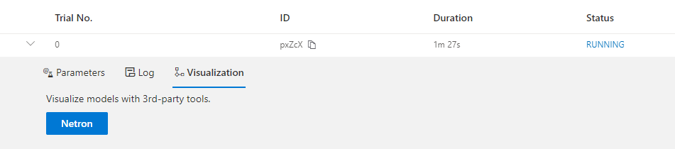
我们支持使用第三方可视化引擎(如 Netron)对模型进行可视化。 这可以通过单击每个试验的详细面板中的“可视化”来使用。 请注意,当前的可视化是基于 onnx, 因此,如果模型不能导出为 onnx,可视化是不可行的。
内置评估器(例如 Classification)会将模型自动导出到文件中。
对于您自己的评估器,您需要将文件保存到 $NNI_OUTPUT_DIR/model.onnx。
例如,
import os
from pathlib import Path


def evaluate_model_with_visualization(model_cls):
    model = model_cls()
    # dump the model into an onnx
    if 'NNI_OUTPUT_DIR' in os.environ:
        dummy_input = torch.zeros(1, 3, 32, 32)
        torch.onnx.export(model, (dummy_input, ),
                          Path(os.environ['NNI_OUTPUT_DIR']) / 'model.onnx')
    evaluate_model(model_cls)
重新启动实验,Web 界面上会显示一个按钮。
导出最优模型
搜索完成后,用户可以使用 export_top_models 导出最优模型。
for model_dict in exp.export_top_models(formatter='dict'):
    print(model_dict)
Out:
{'model_1': '0', 'model_2': 0.25, 'model_3': 64}
输出是一个 JSON 对象,记录了最好的模型的每一个选择都选了什么。 如果用户想要搜出来的模型的源代码,他们可以使用 基于图的引擎,只需增加如下两行。
exp_config.execution_engine = 'base'
export_formatter = 'code'
Total running time of the script: ( 2 minutes 4.499 seconds)