Example Usages of NAS Benchmarks
[3]:
import pprint
import time

from nni.nas.benchmarks.nasbench101 import query_nb101_trial_stats
from nni.nas.benchmarks.nasbench201 import query_nb201_trial_stats
from nni.nas.benchmarks.nds import query_nds_trial_stats

ti = time.time()
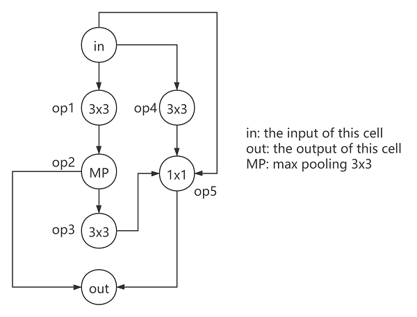
NAS-Bench-101
Use the following architecture as an example:
[2]:
arch = {
    'op1': 'conv3x3-bn-relu',
    'op2': 'maxpool3x3',
    'op3': 'conv3x3-bn-relu',
    'op4': 'conv3x3-bn-relu',
    'op5': 'conv1x1-bn-relu',
    'input1': [0],
    'input2': [1],
    'input3': [2],
    'input4': [0],
    'input5': [0, 3, 4],
    'input6': [2, 5]
}
for t in query_nb101_trial_stats(arch, 108, include_intermediates=True):
    pprint.pprint(t)
An architecture of NAS-Bench-101 could be trained more than once. Each element of the returned generator is a dict which contains one of the training results of this trial config (architecture + hyper-parameters) including train/valid/test accuracy, training time, number of epochs, etc. The results of NAS-Bench-201 and NDS follow similar formats.
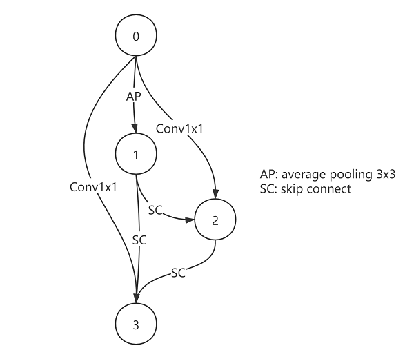
NAS-Bench-201
Use the following architecture as an example:
[3]:
arch = {
    '0_1': 'avg_pool_3x3',
    '0_2': 'conv_1x1',
    '1_2': 'skip_connect',
    '0_3': 'conv_1x1',
    '1_3': 'skip_connect',
    '2_3': 'skip_connect'
}
for t in query_nb201_trial_stats(arch, 200, 'cifar100'):
    pprint.pprint(t)
Intermediate results are also available.
[4]:
for t in query_nb201_trial_stats(arch, None, 'imagenet16-120', include_intermediates=True):
    print(t['config'])
    print('Intermediates:', len(t['intermediates']))
NDS
Use the following architecture as an example: 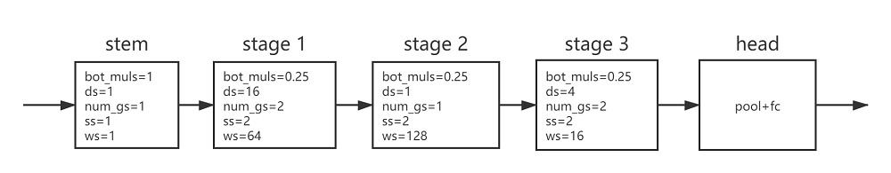
Here, bot_muls, ds, num_gs, ss and ws stand for “bottleneck multipliers”, “depths”, “number of groups”, “strides” and “widths” respectively.
[5]:
model_spec = {
    'bot_muls': [0.0, 0.25, 0.25, 0.25],
    'ds': [1, 16, 1, 4],
    'num_gs': [1, 2, 1, 2],
    'ss': [1, 1, 2, 2],
    'ws': [16, 64, 128, 16]
}
# Use none as a wildcard
for t in query_nds_trial_stats('residual_bottleneck', None, None, model_spec, None, 'cifar10'):
    pprint.pprint(t)
[6]:
model_spec = {
    'bot_muls': [0.0, 0.25, 0.25, 0.25],
    'ds': [1, 16, 1, 4],
    'num_gs': [1, 2, 1, 2],
    'ss': [1, 1, 2, 2],
    'ws': [16, 64, 128, 16]
}
for t in query_nds_trial_stats('residual_bottleneck', None, None, model_spec, None, 'cifar10', include_intermediates=True):
    pprint.pprint(t['intermediates'][:10])
[7]:
model_spec = {'ds': [1, 12, 12, 12], 'ss': [1, 1, 2, 2], 'ws': [16, 24, 24, 40]}
for t in query_nds_trial_stats('residual_basic', 'resnet', 'random', model_spec, {}, 'cifar10'):
    pprint.pprint(t)
[8]:
# get the first one
pprint.pprint(next(query_nds_trial_stats('vanilla', None, None, None, None, None)))
[9]:
# count number
model_spec = {'num_nodes_normal': 5, 'num_nodes_reduce': 5, 'depth': 12, 'width': 32, 'aux': False, 'drop_prob': 0.0}
cell_spec = {
    'normal_0_op_x': 'avg_pool_3x3',
    'normal_0_input_x': 0,
    'normal_0_op_y': 'conv_7x1_1x7',
    'normal_0_input_y': 1,
    'normal_1_op_x': 'sep_conv_3x3',
    'normal_1_input_x': 2,
    'normal_1_op_y': 'sep_conv_5x5',
    'normal_1_input_y': 0,
    'normal_2_op_x': 'dil_sep_conv_3x3',
    'normal_2_input_x': 2,
    'normal_2_op_y': 'dil_sep_conv_3x3',
    'normal_2_input_y': 2,
    'normal_3_op_x': 'skip_connect',
    'normal_3_input_x': 4,
    'normal_3_op_y': 'dil_sep_conv_3x3',
    'normal_3_input_y': 4,
    'normal_4_op_x': 'conv_7x1_1x7',
    'normal_4_input_x': 2,
    'normal_4_op_y': 'sep_conv_3x3',
    'normal_4_input_y': 4,
    'normal_concat': [3, 5, 6],
    'reduce_0_op_x': 'avg_pool_3x3',
    'reduce_0_input_x': 0,
    'reduce_0_op_y': 'dil_sep_conv_3x3',
    'reduce_0_input_y': 1,
    'reduce_1_op_x': 'sep_conv_3x3',
    'reduce_1_input_x': 0,
    'reduce_1_op_y': 'sep_conv_3x3',
    'reduce_1_input_y': 0,
    'reduce_2_op_x': 'skip_connect',
    'reduce_2_input_x': 2,
    'reduce_2_op_y': 'sep_conv_7x7',
    'reduce_2_input_y': 0,
    'reduce_3_op_x': 'conv_7x1_1x7',
    'reduce_3_input_x': 4,
    'reduce_3_op_y': 'skip_connect',
    'reduce_3_input_y': 4,
    'reduce_4_op_x': 'conv_7x1_1x7',
    'reduce_4_input_x': 0,
    'reduce_4_op_y': 'conv_7x1_1x7',
    'reduce_4_input_y': 5,
    'reduce_concat': [3, 6]
}

for t in query_nds_trial_stats('nas_cell', None, None, model_spec, cell_spec, 'cifar10'):
    assert t['config']['model_spec'] == model_spec
    assert t['config']['cell_spec'] == cell_spec
    pprint.pprint(t)
[10]:
# count number
print('NDS (amoeba) count:', len(list(query_nds_trial_stats(None, 'amoeba', None, None, None, None, None))))
NLP
Use the following two architectures as examples. The arch in the paper is called “receipe” with nested variable, and now it is nunested in the benchmarks for NNI. An arch has multiple Node, Node_input_n and Node_op, you can refer to doc for more details.
arch1 : 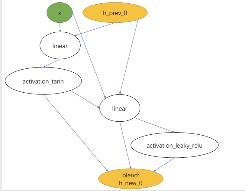
arch2 : 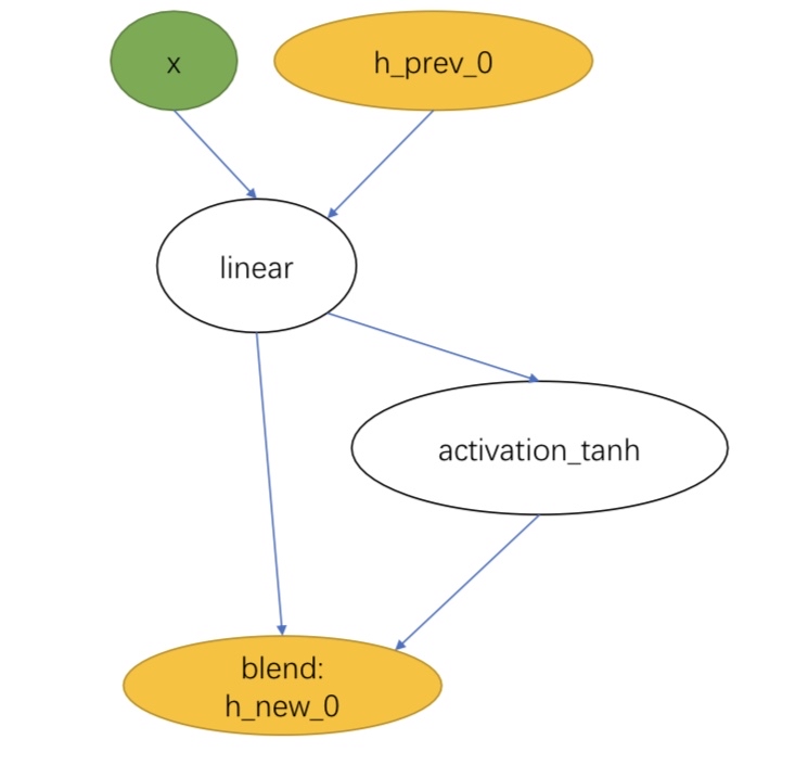
[1]:
import pprint
from nni.nas.benchmarks.nlp import query_nlp_trial_stats

arch1 = {'h_new_0_input_0': 'node_3', 'h_new_0_input_1': 'node_2', 'h_new_0_input_2': 'node_1', 'h_new_0_op': 'blend', 'node_0_input_0': 'x', 'node_0_input_1': 'h_prev_0', 'node_0_op': 'linear','node_1_input_0': 'node_0', 'node_1_op': 'activation_tanh', 'node_2_input_0': 'h_prev_0', 'node_2_input_1': 'node_1', 'node_2_input_2': 'x', 'node_2_op': 'linear', 'node_3_input_0': 'node_2', 'node_3_op': 'activation_leaky_relu'}
for i in query_nlp_trial_stats(arch=arch1, dataset="ptb"):
    pprint.pprint(i)
{'config': {'arch': {'h_new_0_input_0': 'node_3',
                     'h_new_0_input_1': 'node_2',
                     'h_new_0_input_2': 'node_1',
                     'h_new_0_op': 'blend',
                     'node_0_input_0': 'x',
                     'node_0_input_1': 'h_prev_0',
                     'node_0_op': 'linear',
                     'node_1_input_0': 'node_0',
                     'node_1_op': 'activation_tanh',
                     'node_2_input_0': 'h_prev_0',
                     'node_2_input_1': 'node_1',
                     'node_2_input_2': 'x',
                     'node_2_op': 'linear',
                     'node_3_input_0': 'node_2',
                     'node_3_op': 'activation_leaky_relu'},
            'dataset': 'ptb',
            'id': 20003},
 'id': 16291,
 'test_loss': 4.680262297102549,
 'train_loss': 4.132040537087838,
 'training_time': 177.05208373069763,
 'val_loss': 4.707944253177966}
[6]:
arch2 = {"h_new_0_input_0":"node_0","h_new_0_input_1":"node_1","h_new_0_op":"elementwise_sum","node_0_input_0":"x","node_0_input_1":"h_prev_0","node_0_op":"linear","node_1_input_0":"node_0","node_1_op":"activation_tanh"}
for i in query_nlp_trial_stats(arch=arch2, dataset='wikitext-2', include_intermediates=True):
    pprint.pprint(i['intermediates'][45:49])
[{'current_epoch': 46,
  'id': 1796,
  'test_loss': 6.233430054978619,
  'train_loss': 6.4866799231542664,
  'training_time': 146.5680329799652,
  'val_loss': 6.326836978687959},
 {'current_epoch': 47,
  'id': 1797,
  'test_loss': 6.2402057403023825,
  'train_loss': 6.485401405247535,
  'training_time': 146.05511450767517,
  'val_loss': 6.3239741605870865},
 {'current_epoch': 48,
  'id': 1798,
  'test_loss': 6.351145308363877,
  'train_loss': 6.611281181173992,
  'training_time': 145.8849437236786,
  'val_loss': 6.436160816865809},
 {'current_epoch': 49,
  'id': 1799,
  'test_loss': 6.227155079159031,
  'train_loss': 6.473414458249545,
  'training_time': 145.51414465904236,
  'val_loss': 6.313294354607077}]
[4]:
print('Elapsed time: ', time.time() - ti, 'seconds')
Elapsed time: 5.60982608795166 seconds