


Neural Network Intelligence
Overview
NNI (Neural Network Intelligence) is a toolkit to help users design and tune machine learning models (e.g., hyperparameters), neural network architectures, or complex system’s parameters, in an efficient and automatic way. NNI has several appealing properties: ease-of-use, scalability, flexibility, and efficiency.
Ease-of-use: NNI can be easily installed through python pip. Only several lines need to be added to your code in order to use NNI’s power. You can use both the commandline tool and WebUI to work with your experiments.
Scalability: Tuning hyperparameters or the neural architecture often demands a large number of computational resources, while NNI is designed to fully leverage different computation resources, such as remote machines, training platforms (e.g., OpenPAI, Kubernetes). Hundreds of trials could run in parallel by depending on the capacity of your configured training platforms.
Flexibility: Besides rich built-in algorithms, NNI allows users to customize various hyperparameter tuning algorithms, neural architecture search algorithms, early stopping algorithms, etc. Users can also extend NNI with more training platforms, such as virtual machines, kubernetes service on the cloud. Moreover, NNI can connect to external environments to tune special applications/models on them.
Efficiency: We are intensively working on more efficient model tuning on both the system and algorithm level. For example, we leverage early feedback to speedup the tuning procedure.
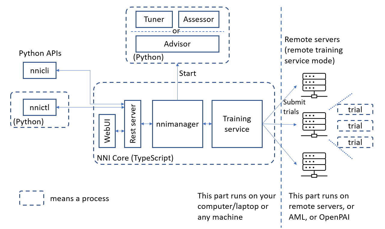
The figure below shows high-level architecture of NNI.
Key Concepts
Experiment: One task of, for example, finding out the best hyperparameters of a model, finding out the best neural network architecture, etc. It consists of trials and AutoML algorithms.
Search Space: The feasible region for tuning the model. For example, the value range of each hyperparameter.
Configuration: An instance from the search space, that is, each hyperparameter has a specific value.
Trial: An individual attempt at applying a new configuration (e.g., a set of hyperparameter values, a specific neural architecture, etc.). Trial code should be able to run with the provided configuration.
Tuner: An AutoML algorithm, which generates a new configuration for the next try. A new trial will run with this configuration.
Assessor: Analyze a trial’s intermediate results (e.g., periodically evaluated accuracy on test dataset) to tell whether this trial can be early stopped or not.
Training Platform: Where trials are executed. Depending on your experiment’s configuration, it could be your local machine, or remote servers, or large-scale training platform (e.g., OpenPAI, Kubernetes).
Basically, an experiment runs as follows: Tuner receives search space and generates configurations. These configurations will be submitted to training platforms, such as the local machine, remote machines, or training clusters. Their performances are reported back to Tuner. Then, new configurations are generated and submitted.
For each experiment, the user only needs to define a search space and update a few lines of code, and then leverage NNI built-in Tuner/Assessor and training platforms to search the best hyperparameters and/or neural architecture. There are basically 3 steps:

For more details about how to run an experiment, please refer to Get Started.
Core Features
NNI provides a key capacity to run multiple instances in parallel to find the best combinations of parameters. This feature can be used in various domains, like finding the best hyperparameters for a deep learning model or finding the best configuration for database and other complex systems with real data.
NNI also provides algorithm toolkits for machine learning and deep learning, especially neural architecture search (NAS) algorithms, model compression algorithms, and feature engineering algorithms.
Hyperparameter Tuning
This is a core and basic feature of NNI, we provide many popular automatic tuning algorithms (i.e., tuner) and early stop algorithms (i.e., assessor). You can follow Quick Start to tune your model (or system). Basically, there are the above three steps and then starting an NNI experiment.
General NAS Framework
This NAS framework is for users to easily specify candidate neural architectures, for example, one can specify multiple candidate operations (e.g., separable conv, dilated conv) for a single layer, and specify possible skip connections. NNI will find the best candidate automatically. On the other hand, the NAS framework provides a simple interface for another type of user (e.g., NAS algorithm researchers) to implement new NAS algorithms. A detailed description of NAS and its usage can be found here.
NNI has support for many one-shot NAS algorithms such as ENAS and DARTS through NNI trial SDK. To use these algorithms you do not have to start an NNI experiment. Instead, import an algorithm in your trial code and simply run your trial code. If you want to tune the hyperparameters in the algorithms or want to run multiple instances, you can choose a tuner and start an NNI experiment.
Other than one-shot NAS, NAS can also run in a classic mode where each candidate architecture runs as an independent trial job. In this mode, similar to hyperparameter tuning, users have to start an NNI experiment and choose a tuner for NAS.
Model Compression
NNI provides an easy-to-use model compression framework to compress deep neural networks, the compressed networks typically have much smaller model size and much faster inference speed without losing performance significantlly. Model compression on NNI includes pruning algorithms and quantization algorithms. NNI provides many pruning and quantization algorithms through NNI trial SDK. Users can directly use them in their trial code and run the trial code without starting an NNI experiment. Users can also use NNI model compression framework to customize their own pruning and quantization algorithms.
A detailed description of model compression and its usage can be found here.
Automatic Feature Engineering
Automatic feature engineering is for users to find the best features for their tasks. A detailed description of automatic feature engineering and its usage can be found here. It is supported through NNI trial SDK, which means you do not have to create an NNI experiment. Instead, simply import a built-in auto-feature-engineering algorithm in your trial code and directly run your trial code.
The auto-feature-engineering algorithms usually have a bunch of hyperparameters themselves. If you want to automatically tune those hyperparameters, you can leverage hyperparameter tuning of NNI, that is, choose a tuning algorithm (i.e., tuner) and start an NNI experiment for it.
Learn More
Installation
Currently we support installation on Linux, Mac and Windows. We also allow you to use docker.
Install on Linux & Mac
Installation
Installation on Linux and macOS follow the same instructions, given below.
Install NNI through pip
Prerequisite:
python 64-bit >= 3.6
python3 -m pip install --upgrade nni
Install NNI through source code
If you are interested in special or the latest code versions, you can install NNI through source code.
Prerequisites:
python 64-bit >=3.6,git
git clone -b v2.5 https://github.com/Microsoft/nni.git
cd nni
python3 -m pip install -U -r dependencies/setup.txt
python3 -m pip install -r dependencies/develop.txt
python3 setup.py develop
Build wheel package from NNI source code
The previous section shows how to install NNI in development mode. If you want to perform a persist install instead, we recommend to build your own wheel package and install from wheel.
git clone -b v2.5 https://github.com/Microsoft/nni.git
cd nni
export NNI_RELEASE=2.0
python3 -m pip install -U -r dependencies/setup.txt
python3 -m pip install -r dependencies/develop.txt
python3 setup.py clean --all
python3 setup.py build_ts
python3 setup.py bdist_wheel -p manylinux1_x86_64
python3 -m pip install dist/nni-2.0-py3-none-manylinux1_x86_64.whl
Use NNI in a docker image
You can also install NNI in a docker image. Please follow the instructions here to build an NNI docker image. The NNI docker image can also be retrieved from Docker Hub through the command
docker pull msranni/nni:latest.
Verify installation
Download the examples via cloning the source code.
git clone -b v2.5 https://github.com/Microsoft/nni.git
Run the MNIST example.
nnictl create --config nni/examples/trials/mnist-pytorch/config.yml
Wait for the message
INFO: Successfully started experiment!in the command line. This message indicates that your experiment has been successfully started. You can explore the experiment using theWeb UI url.
INFO: Starting restful server...
INFO: Successfully started Restful server!
INFO: Setting local config...
INFO: Successfully set local config!
INFO: Starting experiment...
INFO: Successfully started experiment!
-----------------------------------------------------------------------
The experiment id is egchD4qy
The Web UI urls are: http://223.255.255.1:8080 http://127.0.0.1:8080
-----------------------------------------------------------------------
You can use these commands to get more information about the experiment
-----------------------------------------------------------------------
commands description
1. nnictl experiment show show the information of experiments
2. nnictl trial ls list all of trial jobs
3. nnictl top monitor the status of running experiments
4. nnictl log stderr show stderr log content
5. nnictl log stdout show stdout log content
6. nnictl stop stop an experiment
7. nnictl trial kill kill a trial job by id
8. nnictl --help get help information about nnictl
-----------------------------------------------------------------------
Open the
Web UI urlin your browser, you can view detailed information about the experiment and all the submitted trial jobs as shown below. Here are more Web UI pages.


System requirements
Due to potential programming changes, the minimum system requirements of NNI may change over time.
Linux
Recommended |
Minimum |
|
|---|---|---|
Operating System |
Ubuntu 16.04 or above |
|
CPU |
Intel® Core™ i5 or AMD Phenom™ II X3 or better |
Intel® Core™ i3 or AMD Phenom™ X3 8650 |
GPU |
NVIDIA® GeForce® GTX 660 or better |
NVIDIA® GeForce® GTX 460 |
Memory |
6 GB RAM |
4 GB RAM |
Storage |
30 GB available hare drive space |
|
Internet |
Boardband internet connection |
|
Resolution |
1024 x 768 minimum display resolution |
macOS
Recommended |
Minimum |
|
|---|---|---|
Operating System |
macOS 10.14.1 or above |
|
CPU |
Intel® Core™ i7-4770 or better |
Intel® Core™ i5-760 or better |
GPU |
AMD Radeon™ R9 M395X or better |
NVIDIA® GeForce® GT 750M or AMD Radeon™ R9 M290 or better |
Memory |
8 GB RAM |
4 GB RAM |
Storage |
70GB available space SSD |
70GB available space 7200 RPM HDD |
Internet |
Boardband internet connection |
|
Resolution |
1024 x 768 minimum display resolution |
Further reading
Install on Windows
Prerequires
Python 3.6 (or above) 64-bit. Anaconda or Miniconda is highly recommended to manage multiple Python environments on Windows.
If it’s a newly installed Python environment, it needs to install Microsoft C++ Build Tools to support build NNI dependencies like
scikit-learn.pip install cython wheel
git for verifying installation.
Install NNI
In most cases, you can install and upgrade NNI from pip package. It’s easy and fast.
If you are interested in special or the latest code versions, you can install NNI through source code.
If you want to contribute to NNI, refer to setup development environment.
From pip package
python -m pip install --upgrade nni
From source code
git clone -b v2.5 https://github.com/Microsoft/nni.git cd nni python -m pip install -U -r dependencies/setup.txt python -m pip install -r dependencies/develop.txt python setup.py develop
Verify installation
Clone examples within source code.
git clone -b v2.5 https://github.com/Microsoft/nni.git
Run the MNIST example.
nnictl create --config nni\examples\trials\mnist-pytorch\config_windows.yml Note: If you are familiar with other frameworks, you can choose corresponding example under ``examples\trials``. It needs to change trial command ``python3`` to ``python`` in each example YAML, since default installation has ``python.exe``\ , not ``python3.exe`` executable.
Wait for the message
INFO: Successfully started experiment!in the command line. This message indicates that your experiment has been successfully started. You can explore the experiment using theWeb UI url.
INFO: Starting restful server...
INFO: Successfully started Restful server!
INFO: Setting local config...
INFO: Successfully set local config!
INFO: Starting experiment...
INFO: Successfully started experiment!
-----------------------------------------------------------------------
The experiment id is egchD4qy
The Web UI urls are: http://223.255.255.1:8080 http://127.0.0.1:8080
-----------------------------------------------------------------------
You can use these commands to get more information about the experiment
-----------------------------------------------------------------------
commands description
1. nnictl experiment show show the information of experiments
2. nnictl trial ls list all of trial jobs
3. nnictl top monitor the status of running experiments
4. nnictl log stderr show stderr log content
5. nnictl log stdout show stdout log content
6. nnictl stop stop an experiment
7. nnictl trial kill kill a trial job by id
8. nnictl --help get help information about nnictl
-----------------------------------------------------------------------
Open the
Web UI urlin your browser, you can view detailed information about the experiment and all the submitted trial jobs as shown below. Here are more Web UI pages.
System requirements
Below are the minimum system requirements for NNI on Windows, Windows 10.1809 is well tested and recommend. Due to potential programming changes, the minimum system requirements for NNI may change over time.
Recommended |
Minimum |
|
|---|---|---|
Operating System |
Windows 10 1809 or above |
|
CPU |
Intel® Core™ i5 or AMD Phenom™ II X3 or better |
Intel® Core™ i3 or AMD Phenom™ X3 8650 |
GPU |
NVIDIA® GeForce® GTX 660 or better |
NVIDIA® GeForce® GTX 460 |
Memory |
6 GB RAM |
4 GB RAM |
Storage |
30 GB available hare drive space |
|
Internet |
Boardband internet connection |
|
Resolution |
1024 x 768 minimum display resolution |
FAQ
simplejson failed when installing NNI
Make sure a C++ 14.0 compiler is installed.
building ‘simplejson._speedups’ extension error: [WinError 3] The system cannot find the path specified
Trial failed with missing DLL in command line or PowerShell
This error is caused by missing LIBIFCOREMD.DLL and LIBMMD.DLL and failure to install SciPy. Using Anaconda or Miniconda with Python(64-bit) can solve it.
ImportError: DLL load failed
Trial failed on webUI
Please check the trial log file stderr for more details.
If there is a stderr file, please check it. Two possible cases are:
forgetting to change the trial command
python3topythonin each experiment YAML.forgetting to install experiment dependencies such as TensorFlow, Keras and so on.
Fail to use BOHB on Windows
Make sure a C++ 14.0 compiler is installed when trying to run pip install nni[BOHB] to install the dependencies.
Not supported tuner on Windows
SMAC is not supported currently; for the specific reason refer to this GitHub issue.
Use Windows as a remote worker
Refer to Remote Machine mode.
Segmentation fault (core dumped) when installing
Refer to FAQ.
Further reading
How to Use Docker in NNI
Overview
Docker is a tool to make it easier for users to deploy and run applications based on their own operating system by starting containers. Docker is not a virtual machine, it does not create a virtual operating system, but it allows different applications to use the same OS kernel and isolate different applications by container.
Users can start NNI experiments using Docker. NNI also provides an official Docker image msranni/nni on Docker Hub.
Using Docker in local machine
Step 1: Installation of Docker
Before you start using Docker for NNI experiments, you should install Docker on your local machine. See here.
Step 2: Start a Docker container
If you have installed the Docker package in your local machine, you can start a Docker container instance to run NNI examples. You should notice that because NNI will start a web UI process in a container and continue to listen to a port, you need to specify the port mapping between your host machine and Docker container to give access to web UI outside the container. By visiting the host IP address and port, you can redirect to the web UI process started in Docker container and visit web UI content.
For example, you could start a new Docker container from the following command:
docker run -i -t -p [hostPort]:[containerPort] [image]
-i: Start a Docker in an interactive mode.
-t: Docker assign the container an input terminal.
-p: Port mapping, map host port to a container port.
For more information about Docker commands, please refer to this.
Note:
NNI only supports Ubuntu and MacOS systems in local mode for the moment, please use correct Docker image type. If you want to use gpu in a Docker container, please use nvidia-docker.
Step 3: Run NNI in a Docker container
If you start a Docker image using NNI’s official image msranni/nni, you can directly start NNI experiments by using the nnictl command. Our official image has NNI’s running environment and basic python and deep learning frameworks preinstalled.
If you start your own Docker image, you may need to install the NNI package first; please refer to NNI installation.
If you want to run NNI’s official examples, you may need to clone the NNI repo in GitHub using
git clone https://github.com/Microsoft/nni.git
then you can enter nni/examples/trials to start an experiment.
After you prepare NNI’s environment, you can start a new experiment using the nnictl command. See here.
Using Docker on a remote platform
NNI supports starting experiments in remoteTrainingService, and running trial jobs on remote machines. As Docker can start an independent Ubuntu system as an SSH server, a Docker container can be used as the remote machine in NNI’s remote mode.
Step 1: Setting a Docker environment
You should install the Docker software on your remote machine first, please refer to this.
To make sure your Docker container can be connected by NNI experiments, you should build your own Docker image to set an SSH server or use images with an SSH configuration. If you want to use a Docker container as an SSH server, you should configure the SSH password login or private key login; please refer to this.
Note:
NNI's official image msranni/nni does not support SSH servers for the time being; you should build your own Docker image with an SSH configuration or use other images as a remote server.
Step 2: Start a Docker container on a remote machine
An SSH server needs a port; you need to expose Docker’s SSH port to NNI as the connection port. For example, if you set your container’s SSH port as A, you should map the container’s port A to your remote host machine’s other port B, NNI will connect port B as an SSH port, and your host machine will map the connection from port B to port A then NNI could connect to your Docker container.
For example, you could start your Docker container using the following commands:
docker run -dit -p [hostPort]:[containerPort] [image]
The containerPort is the SSH port used in your Docker container and the hostPort is your host machine’s port exposed to NNI. You can set your NNI’s config file to connect to hostPort and the connection will be transmitted to your Docker container.
For more information about Docker commands, please refer to this.
Note:
If you use your own Docker image as a remote server, please make sure that this image has a basic python environment and an NNI SDK runtime environment. If you want to use a GPU in a Docker container, please use nvidia-docker.
Step 3: Run NNI experiments
You can set your config file as a remote platform and set the machineList configuration to connect to your Docker SSH server; refer to this. Note that you should set the correct port, username, and passWd or sshKeyPath of your host machine.
port: The host machine’s port, mapping to Docker’s SSH port.
username: The username of the Docker container.
passWd: The password of the Docker container.
sshKeyPath: The path of the private key of the Docker container.
After the configuration of the config file, you could start an experiment, refer to this.
QuickStart
Installation
Currently, NNI supports running on Linux, macOS and Windows. Ubuntu 16.04 or higher, macOS 10.14.1, and Windows 10.1809 are tested and supported. Simply run the following pip install in an environment that has python >= 3.6.
Linux and macOS
python3 -m pip install --upgrade nni
Windows
python -m pip install --upgrade nni
Note
For Linux and macOS, --user can be added if you want to install NNI in your home directory, which does not require any special privileges.
Note
If there is an error like Segmentation fault, please refer to the FAQ.
Note
For the system requirements of NNI, please refer to Install NNI on Linux & Mac or Windows. If you want to use docker, refer to HowToUseDocker.
“Hello World” example on MNIST
NNI is a toolkit to help users run automated machine learning experiments. It can automatically do the cyclic process of getting hyperparameters, running trials, testing results, and tuning hyperparameters. Here, we’ll show how to use NNI to help you find the optimal hyperparameters on the MNIST dataset.
Here is an example script to train a CNN on the MNIST dataset without NNI:
def main(args):
# load data
train_loader = torch.utils.data.DataLoader(datasets.MNIST(...), batch_size=args['batch_size'], shuffle=True)
test_loader = torch.tuils.data.DataLoader(datasets.MNIST(...), batch_size=1000, shuffle=True)
# build model
model = Net(hidden_size=args['hidden_size'])
optimizer = optim.SGD(model.parameters(), lr=args['lr'], momentum=args['momentum'])
# train
for epoch in range(10):
train(args, model, device, train_loader, optimizer, epoch)
test_acc = test(args, model, device, test_loader)
print(test_acc)
print('final accuracy:', test_acc)
if __name__ == '__main__':
params = {
'batch_size': 32,
'hidden_size': 128,
'lr': 0.001,
'momentum': 0.5
}
main(params)
The above code can only try one set of parameters at a time. If you want to tune the learning rate, you need to manually modify the hyperparameter and start the trial again and again.
NNI is born to help users tune jobs, whose working process is presented below:
input: search space, trial code, config file
output: one optimal hyperparameter configuration
1: For t = 0, 1, 2, ..., maxTrialNum,
2: hyperparameter = chose a set of parameter from search space
3: final result = run_trial_and_evaluate(hyperparameter)
4: report final result to NNI
5: If reach the upper limit time,
6: Stop the experiment
7: return hyperparameter value with best final result
Note
If you want to use NNI to automatically train your model and find the optimal hyper-parameters, there are two approaches:
Write a config file and start the experiment from the command line.
Config and launch the experiment directly from a Python file
In the this part, we will focus on the first approach. For the second approach, please refer to this tutorial.
Step 1: Modify the Trial Code
Modify your Trial file to get the hyperparameter set from NNI and report the final results to NNI.
+ import nni
def main(args):
# load data
train_loader = torch.utils.data.DataLoader(datasets.MNIST(...), batch_size=args['batch_size'], shuffle=True)
test_loader = torch.tuils.data.DataLoader(datasets.MNIST(...), batch_size=1000, shuffle=True)
# build model
model = Net(hidden_size=args['hidden_size'])
optimizer = optim.SGD(model.parameters(), lr=args['lr'], momentum=args['momentum'])
# train
for epoch in range(10):
train(args, model, device, train_loader, optimizer, epoch)
test_acc = test(args, model, device, test_loader)
- print(test_acc)
+ nni.report_intermediate_result(test_acc)
- print('final accuracy:', test_acc)
+ nni.report_final_result(test_acc)
if __name__ == '__main__':
- params = {'batch_size': 32, 'hidden_size': 128, 'lr': 0.001, 'momentum': 0.5}
+ params = nni.get_next_parameter()
main(params)
Example: mnist.py
Step 2: Define the Search Space
Define a Search Space in a YAML file, including the name and the distribution (discrete-valued or continuous-valued) of all the hyperparameters you want to search.
searchSpace:
batch_size:
_type: choice
_value: [16, 32, 64, 128]
hidden_size:
_type: choice
_value: [128, 256, 512, 1024]
lr:
_type: choice
_value: [0.0001, 0.001, 0.01, 0.1]
momentum:
_type: uniform
_value: [0, 1]
Example: config_detailed.yml
You can also write your search space in a JSON file and specify the file path in the configuration. For detailed tutorial on how to write the search space, please see here.
Step 3: Config the Experiment
In addition to the search_space defined in the step2, you need to config the experiment in the YAML file. It specifies the key information of the experiment, such as the trial files, tuning algorithm, max trial number, and max duration, etc.
experimentName: MNIST # An optional name to distinguish the experiments
trialCommand: python3 mnist.py # NOTE: change "python3" to "python" if you are using Windows
trialConcurrency: 2 # Run 2 trials concurrently
maxTrialNumber: 10 # Generate at most 10 trials
maxExperimentDuration: 1h # Stop generating trials after 1 hour
tuner: # Configure the tuning algorithm
name: TPE
classArgs: # Algorithm specific arguments
optimize_mode: maximize
trainingService: # Configure the training platform
platform: local
Experiment config reference could be found here.
Note
If you are planning to use remote machines or clusters as your training service, to avoid too much pressure on network, NNI limits the number of files to 2000 and total size to 300MB. If your codeDir contains too many files, you can choose which files and subfolders should be excluded by adding a .nniignore file that works like a .gitignore file. For more details on how to write this file, see the git documentation.
Example: config_detailed.yml and .nniignore
All the code above is already prepared and stored in examples/trials/mnist-pytorch/.
Step 4: Launch the Experiment
Linux and macOS
Run the config_detailed.yml file from your command line to start the experiment.
nnictl create --config nni/examples/trials/mnist-pytorch/config_detailed.yml
Windows
Change python3 to python of the trialCommand field in the config_detailed.yml file, and run the config_detailed.yml file from your command line to start the experiment.
nnictl create --config nni\examples\trials\mnist-pytorch\config_detailed.yml
Note
nnictl is a command line tool that can be used to control experiments, such as start/stop/resume an experiment, start/stop NNIBoard, etc. Click here for more usage of nnictl.
Wait for the message INFO: Successfully started experiment! in the command line. This message indicates that your experiment has been successfully started. And this is what we expect to get:
INFO: Starting restful server...
INFO: Successfully started Restful server!
INFO: Setting local config...
INFO: Successfully set local config!
INFO: Starting experiment...
INFO: Successfully started experiment!
-----------------------------------------------------------------------
The experiment id is egchD4qy
The Web UI urls are: [Your IP]:8080
-----------------------------------------------------------------------
You can use these commands to get more information about the experiment
-----------------------------------------------------------------------
commands description
1. nnictl experiment show show the information of experiments
2. nnictl trial ls list all of trial jobs
3. nnictl top monitor the status of running experiments
4. nnictl log stderr show stderr log content
5. nnictl log stdout show stdout log content
6. nnictl stop stop an experiment
7. nnictl trial kill kill a trial job by id
8. nnictl --help get help information about nnictl
-----------------------------------------------------------------------
If you prepared trial, search space, and config according to the above steps and successfully created an NNI job, NNI will automatically tune the optimal hyper-parameters and run different hyper-parameter sets for each trial according to the defined search space. You can see its progress through the WebUI clearly.
Step 5: View the Experiment
After starting the experiment successfully, you can find a message in the command-line interface that tells you the Web UI url like this:
The Web UI urls are: [Your IP]:8080
Open the Web UI url (Here it’s: [Your IP]:8080) in your browser, you can view detailed information about the experiment and all the submitted trial jobs as shown below. If you cannot open the WebUI link in your terminal, please refer to the FAQ.
View Overview Page
Information about this experiment will be shown in the WebUI, including the experiment profile and search space message. NNI also supports downloading this information and the parameters through the Experiment summary button.

View Trials Detail Page
You could see the best trial metrics and hyper-parameter graph in this page. And the table content includes more columns when you click the button Add/Remove columns.

View Experiments Management Page
On the All experiments page, you can see all the experiments on your machine.

For more detailed usage of WebUI, please refer to this doc.
Auto (Hyper-parameter) Tuning
Auto tuning is one of the key features provided by NNI; a main application scenario being hyper-parameter tuning. Tuning specifically applies to trial code. We provide a lot of popular auto tuning algorithms (called Tuner), and some early stop algorithms (called Assessor). NNI supports running trials on various training platforms, for example, on a local machine, on several servers in a distributed manner, or on platforms such as OpenPAI, Kubernetes, etc.
Other key features of NNI, such as model compression, feature engineering, can also be further enhanced by auto tuning, which we’ll described when introducing those features.
NNI has high extensibility, advanced users can customize their own Tuner, Assessor, and Training Service according to their needs.
Write a Trial Run on NNI
A Trial in NNI is an individual attempt at applying a configuration (e.g., a set of hyper-parameters) to a model.
To define an NNI trial, you need to first define the set of parameters (i.e., search space) and then update the model. NNI provides two approaches for you to define a trial: NNI API and NNI Python annotation. You could also refer to here for more trial examples.
NNI API
Step 1 - Prepare a SearchSpace parameters file.
An example is shown below:
{
"dropout_rate":{"_type":"uniform","_value":[0.1,0.5]},
"conv_size":{"_type":"choice","_value":[2,3,5,7]},
"hidden_size":{"_type":"choice","_value":[124, 512, 1024]},
"learning_rate":{"_type":"uniform","_value":[0.0001, 0.1]}
}
Refer to SearchSpaceSpec to learn more about search spaces. Tuner will generate configurations from this search space, that is, choosing a value for each hyperparameter from the range.
Step 2 - Update model code
Import NNI
Include
import nniin your trial code to use NNI APIs.Get configuration from Tuner
RECEIVED_PARAMS = nni.get_next_parameter()
RECEIVED_PARAMS is an object, for example:
{"conv_size": 2, "hidden_size": 124, "learning_rate": 0.0307, "dropout_rate": 0.2029}.
Report metric data periodically (optional)
nni.report_intermediate_result(metrics)
metrics can be any python object. If users use the NNI built-in tuner/assessor, metrics can only have two formats: 1) a number e.g., float, int, or 2) a dict object that has a key named default whose value is a number. These metrics are reported to assessor. Often, metrics includes the periodically evaluated loss or accuracy.
Report performance of the configuration
nni.report_final_result(metrics)
metrics can also be any python object. If users use the NNI built-in tuner/assessor, metrics follows the same format rule as that in report_intermediate_result, the number indicates the model’s performance, for example, the model’s accuracy, loss etc. These metrics are reported to tuner.
Step 3 - Enable NNI API
To enable NNI API mode, you need to set useAnnotation to false and provide the path of the SearchSpace file was defined in step 1:
useAnnotation: false
searchSpacePath: /path/to/your/search_space.json
You can refer to here for more information about how to set up experiment configurations.
Please refer to here for more APIs (e.g., nni.get_sequence_id()) provided by NNI.
NNI Python Annotation
An alternative to writing a trial is to use NNI’s syntax for python. NNI annotations are simple, similar to comments. You don’t have to make structural changes to your existing code. With a few lines of NNI annotation, you will be able to:
annotate the variables you want to tune
specify the range in which you want to tune the variables
annotate which variable you want to report as an intermediate result to
assessorannotate which variable you want to report as the final result (e.g. model accuracy) to
tuner.
Again, take MNIST as an example, it only requires 2 steps to write a trial with NNI Annotation.
Step 1 - Update codes with annotations
The following is a TensorFlow code snippet for NNI Annotation where the highlighted four lines are annotations that:
tune batch_size and dropout_rate
report test_acc every 100 steps
lastly report test_acc as the final result.
It’s worth noting that, as these newly added codes are merely annotations, you can still run your code as usual in environments without NNI installed.
with tf.Session() as sess:
sess.run(tf.global_variables_initializer())
+ """@nni.variable(nni.choice(50, 250, 500), name=batch_size)"""
batch_size = 128
for i in range(10000):
batch = mnist.train.next_batch(batch_size)
+ """@nni.variable(nni.choice(0.1, 0.5), name=dropout_rate)"""
dropout_rate = 0.5
mnist_network.train_step.run(feed_dict={mnist_network.images: batch[0],
mnist_network.labels: batch[1],
mnist_network.keep_prob: dropout_rate})
if i % 100 == 0:
test_acc = mnist_network.accuracy.eval(
feed_dict={mnist_network.images: mnist.test.images,
mnist_network.labels: mnist.test.labels,
mnist_network.keep_prob: 1.0})
+ """@nni.report_intermediate_result(test_acc)"""
test_acc = mnist_network.accuracy.eval(
feed_dict={mnist_network.images: mnist.test.images,
mnist_network.labels: mnist.test.labels,
mnist_network.keep_prob: 1.0})
+ """@nni.report_final_result(test_acc)"""
NOTE:
@nni.variablewill affect its following line which should be an assignment statement whose left-hand side must be the same as the keywordnamein the@nni.variablestatement.@nni.report_intermediate_result/@nni.report_final_resultwill send the data to assessor/tuner at that line.
For more information about annotation syntax and its usage, please refer to Annotation.
Step 2 - Enable NNI Annotation
In the YAML configure file, you need to set useAnnotation to true to enable NNI annotation:
useAnnotation: true
Standalone mode for debugging
NNI supports a standalone mode for trial code to run without starting an NNI experiment. This is for finding out bugs in trial code more conveniently. NNI annotation natively supports standalone mode, as the added NNI related lines are comments. For NNI trial APIs, the APIs have changed behaviors in standalone mode, some APIs return dummy values, and some APIs do not really report values. Please refer to the following table for the full list of these APIs.
# NOTE: please assign default values to the hyperparameters in your trial code
nni.get_next_parameter # return {}
nni.report_final_result # have log printed on stdout, but does not report
nni.report_intermediate_result # have log printed on stdout, but does not report
nni.get_experiment_id # return "STANDALONE"
nni.get_trial_id # return "STANDALONE"
nni.get_sequence_id # return 0
You can try standalone mode with the mnist example. Simply run python3 mnist.py under the code directory. The trial code should successfully run with the default hyperparameter values.
For more information on debugging, please refer to How to Debug
Where are my trials?
Local Mode
In NNI, every trial has a dedicated directory for them to output their own data. In each trial, an environment variable called NNI_OUTPUT_DIR is exported. Under this directory, you can find each trial’s code, data, and other logs. In addition, each trial’s log (including stdout) will be re-directed to a file named trial.log under that directory.
If NNI Annotation is used, the trial’s converted code is in another temporary directory. You can check that in a file named run.sh under the directory indicated by NNI_OUTPUT_DIR. The second line (i.e., the cd command) of this file will change directory to the actual directory where code is located. Below is an example of run.sh:
#!/bin/bash
cd /tmp/user_name/nni/annotation/tmpzj0h72x6 #This is the actual directory
export NNI_PLATFORM=local
export NNI_SYS_DIR=/home/user_name/nni-experiments/$experiment_id$/trials/$trial_id$
export NNI_TRIAL_JOB_ID=nrbb2
export NNI_OUTPUT_DIR=/home/user_name/nni-experiments/$eperiment_id$/trials/$trial_id$
export NNI_TRIAL_SEQ_ID=1
export MULTI_PHASE=false
export CUDA_VISIBLE_DEVICES=
eval python3 mnist.py 2>/home/user_name/nni-experiments/$experiment_id$/trials/$trial_id$/stderr
echo $? `date +%s%3N` >/home/user_name/nni-experiments/$experiment_id$/trials/$trial_id$/.nni/state
Other Modes
When running trials on other platforms like remote machine or PAI, the environment variable NNI_OUTPUT_DIR only refers to the output directory of the trial, while the trial code and run.sh might not be there. However, the trial.log will be transmitted back to the local machine in the trial’s directory, which defaults to ~/nni-experiments/$experiment_id$/trials/$trial_id$/
For more information, please refer to HowToDebug.
More Trial Examples
Builtin-Tuners
NNI provides an easy way to adopt an approach to set up parameter tuning algorithms, we call them Tuner.
Tuner receives metrics from Trial to evaluate the performance of a specific parameters/architecture configuration. Tuner sends the next hyper-parameter or architecture configuration to Trial.
HyperParameter Tuning with NNI Built-in Tuners
To fit a machine/deep learning model into different tasks/problems, hyperparameters always need to be tuned. Automating the process of hyperparaeter tuning always requires a good tuning algorithm. NNI has provided state-of-the-art tuning algorithms as part of our built-in tuners and makes them easy to use. Below is the brief summary of NNI’s current built-in tuners:
Note: Click the Tuner’s name to get the Tuner’s installation requirements, suggested scenario, and an example configuration. A link for a detailed description of each algorithm is located at the end of the suggested scenario for each tuner. Here is an article comparing different Tuners on several problems.
Currently, we support the following algorithms:
Tuner |
Brief Introduction of Algorithm |
|---|---|
The Tree-structured Parzen Estimator (TPE) is a sequential model-based optimization (SMBO) approach. SMBO methods sequentially construct models to approximate the performance of hyperparameters based on historical measurements, and then subsequently choose new hyperparameters to test based on this model. Reference Paper |
|
In Random Search for Hyper-Parameter Optimization show that Random Search might be surprisingly simple and effective. We suggest that we could use Random Search as the baseline when we have no knowledge about the prior distribution of hyper-parameters. Reference Paper |
|
This simple annealing algorithm begins by sampling from the prior, but tends over time to sample from points closer and closer to the best ones observed. This algorithm is a simple variation on the random search that leverages smoothness in the response surface. The annealing rate is not adaptive. |
|
Naïve Evolution comes from Large-Scale Evolution of Image Classifiers. It randomly initializes a population-based on search space. For each generation, it chooses better ones and does some mutation (e.g., change a hyperparameter, add/remove one layer) on them to get the next generation. Naïve Evolution requires many trials to work, but it’s very simple and easy to expand new features. Reference paper |
|
SMAC is based on Sequential Model-Based Optimization (SMBO). It adapts the most prominent previously used model class (Gaussian stochastic process models) and introduces the model class of random forests to SMBO, in order to handle categorical parameters. The SMAC supported by NNI is a wrapper on the SMAC3 GitHub repo. Notice, SMAC needs to be installed by |
|
Batch tuner allows users to simply provide several configurations (i.e., choices of hyper-parameters) for their trial code. After finishing all the configurations, the experiment is done. Batch tuner only supports the type choice in search space spec. |
|
Grid Search performs an exhaustive searching through a manually specified subset of the hyperparameter space defined in the searchspace file. Note that the only acceptable types of search space are choice, quniform, randint. |
|
Hyperband tries to use limited resources to explore as many configurations as possible and returns the most promising ones as a final result. The basic idea is to generate many configurations and run them for a small number of trials. The half least-promising configurations are thrown out, the remaining are further trained along with a selection of new configurations. The size of these populations is sensitive to resource constraints (e.g. allotted search time). Reference Paper |
|
Network Morphism provides functions to automatically search for deep learning architectures. It generates child networks that inherit the knowledge from their parent network which it is a morph from. This includes changes in depth, width, and skip-connections. Next, it estimates the value of a child network using historic architecture and metric pairs. Then it selects the most promising one to train. Reference Paper |
|
Metis offers the following benefits when it comes to tuning parameters: While most tools only predict the optimal configuration, Metis gives you two outputs: (a) current prediction of optimal configuration, and (b) suggestion for the next trial. No more guesswork. While most tools assume training datasets do not have noisy data, Metis actually tells you if you need to re-sample a particular hyper-parameter. Reference Paper |
|
BOHB is a follow-up work to Hyperband. It targets the weakness of Hyperband that new configurations are generated randomly without leveraging finished trials. For the name BOHB, HB means Hyperband, BO means Bayesian Optimization. BOHB leverages finished trials by building multiple TPE models, a proportion of new configurations are generated through these models. Reference Paper |
|
Gaussian Process Tuner is a sequential model-based optimization (SMBO) approach with Gaussian Process as the surrogate. Reference Paper, Github Repo |
|
PBT Tuner is a simple asynchronous optimization algorithm which effectively utilizes a fixed computational budget to jointly optimize a population of models and their hyperparameters to maximize performance. Reference Paper |
|
Use of neural networks as an alternative to GPs to model distributions over functions in bayesian optimization. |
Usage of Built-in Tuners
Using a built-in tuner provided by the NNI SDK requires one to declare the builtinTunerName and classArgs in the config.yml file. In this part, we will introduce each tuner along with information about usage and suggested scenarios, classArg requirements, and an example configuration.
Note: Please follow the format when you write your config.yml file. Some built-in tuners have dependencies that need to be installed using pip install nni[<tuner>], like SMAC’s dependencies can be installed using pip install nni[SMAC].
TPE
Built-in Tuner Name: TPE
Suggested scenario
TPE, as a black-box optimization, can be used in various scenarios and shows good performance in general. Especially when you have limited computation resources and can only try a small number of trials. From a large amount of experiments, we found that TPE is far better than Random Search. Detailed Description
classArgs Requirements:
optimize_mode (maximize or minimize, optional, default = maximize) - If ‘maximize’, the tuner will try to maximize metrics. If ‘minimize’, the tuner will try to minimize metrics.
Note: We have optimized the parallelism of TPE for large-scale trial concurrency. For the principle of optimization or turn-on optimization, please refer to TPE document.
Example Configuration:
# config.yml
tuner:
builtinTunerName: TPE
classArgs:
optimize_mode: maximize
Random Search
Built-in Tuner Name: Random
Suggested scenario
Random search is suggested when each trial does not take very long (e.g., each trial can be completed very quickly, or early stopped by the assessor), and you have enough computational resources. It’s also useful if you want to uniformly explore the search space. Random Search can be considered a baseline search algorithm. Detailed Description
Example Configuration:
# config.yml
tuner:
builtinTunerName: Random
Anneal
Built-in Tuner Name: Anneal
Suggested scenario
Anneal is suggested when each trial does not take very long and you have enough computation resources (very similar to Random Search). It’s also useful when the variables in the search space can be sample from some prior distribution. Detailed Description
classArgs Requirements:
optimize_mode (maximize or minimize, optional, default = maximize) - If ‘maximize’, the tuner will try to maximize metrics. If ‘minimize’, the tuner will try to minimize metrics.
Example Configuration:
# config.yml
tuner:
builtinTunerName: Anneal
classArgs:
optimize_mode: maximize
Naïve Evolution
Built-in Tuner Name: Evolution
Suggested scenario
Its computational resource requirements are relatively high. Specifically, it requires a large initial population to avoid falling into a local optimum. If your trial is short or leverages assessor, this tuner is a good choice. It is also suggested when your trial code supports weight transfer; that is, the trial could inherit the converged weights from its parent(s). This can greatly speed up the training process. Detailed Description
classArgs Requirements:
optimize_mode (maximize or minimize, optional, default = maximize) - If ‘maximize’, the tuner will try to maximize metrics. If ‘minimize’, the tuner will try to minimize metrics.
population_size (int value (should > 0), optional, default = 20) - the initial size of the population (trial num) in the evolution tuner. It’s suggested that
population_sizebe much larger thanconcurrencyso users can get the most out of the algorithm (and at leastconcurrency, or the tuner will fail on its first generation of parameters).
Example Configuration:
# config.yml
tuner:
builtinTunerName: Evolution
classArgs:
optimize_mode: maximize
population_size: 100
SMAC
Built-in Tuner Name: SMAC
Please note that SMAC doesn’t support running on Windows currently. For the specific reason, please refer to this GitHub issue.
Installation
SMAC has dependencies that need to be installed by following command before the first usage. As a reminder, swig is required for SMAC: for Ubuntu swig can be installed with apt.
pip install nni[SMAC]
Suggested scenario
Similar to TPE, SMAC is also a black-box tuner that can be tried in various scenarios and is suggested when computational resources are limited. It is optimized for discrete hyperparameters, thus, it’s suggested when most of your hyperparameters are discrete. Detailed Description
classArgs Requirements:
optimize_mode (maximize or minimize, optional, default = maximize) - If ‘maximize’, the tuner will try to maximize metrics. If ‘minimize’, the tuner will try to minimize metrics.
config_dedup (True or False, optional, default = False) - If True, the tuner will not generate a configuration that has been already generated. If False, a configuration may be generated twice, but it is rare for a relatively large search space.
Example Configuration:
# config.yml
tuner:
builtinTunerName: SMAC
classArgs:
optimize_mode: maximize
Batch Tuner
Built-in Tuner Name: BatchTuner
Suggested scenario
If the configurations you want to try have been decided beforehand, you can list them in search space file (using choice) and run them using batch tuner. Detailed Description
Example Configuration:
# config.yml
tuner:
builtinTunerName: BatchTuner
Note that the search space for BatchTuner should look like:
{
"combine_params":
{
"_type" : "choice",
"_value" : [{"optimizer": "Adam", "learning_rate": 0.00001},
{"optimizer": "Adam", "learning_rate": 0.0001},
{"optimizer": "Adam", "learning_rate": 0.001},
{"optimizer": "SGD", "learning_rate": 0.01},
{"optimizer": "SGD", "learning_rate": 0.005},
{"optimizer": "SGD", "learning_rate": 0.0002}]
}
}
The search space file should include the high-level key combine_params. The type of params in the search space must be choice and the values must include all the combined params values.
Grid Search
Built-in Tuner Name: Grid Search
Suggested scenario
Note that the only acceptable types within the search space are choice, quniform, and randint.
This is suggested when the search space is small. It’s suggested when it is feasible to exhaustively sweep the whole search space. Detailed Description
Example Configuration:
# config.yml
tuner:
builtinTunerName: GridSearch
Hyperband
Built-in Advisor Name: Hyperband
Suggested scenario
This is suggested when you have limited computational resources but have a relatively large search space. It performs well in scenarios where intermediate results can indicate good or bad final results to some extent. For example, when models that are more accurate early on in training are also more accurate later on. Detailed Description
classArgs Requirements:
optimize_mode (maximize or minimize, optional, default = maximize) - If ‘maximize’, the tuner will try to maximize metrics. If ‘minimize’, the tuner will try to minimize metrics.
R (int, optional, default = 60) - the maximum budget given to a trial (could be the number of mini-batches or epochs). Each trial should use TRIAL_BUDGET to control how long they run.
eta (int, optional, default = 3) -
(eta-1)/etais the proportion of discarded trials.exec_mode (serial or parallelism, optional, default = parallelism) - If ‘parallelism’, the tuner will try to use available resources to start new bucket immediately. If ‘serial’, the tuner will only start new bucket after the current bucket is done.
Example Configuration:
# config.yml
advisor:
builtinAdvisorName: Hyperband
classArgs:
optimize_mode: maximize
R: 60
eta: 3
Network Morphism
Built-in Tuner Name: NetworkMorphism
Installation
NetworkMorphism requires PyTorch.
Suggested scenario
This is suggested when you want to apply deep learning methods to your task but you have no idea how to choose or design a network. You may modify this example to fit your own dataset and your own data augmentation method. Also you can change the batch size, learning rate, or optimizer. Currently, this tuner only supports the computer vision domain. Detailed Description
classArgs Requirements:
optimize_mode (maximize or minimize, optional, default = maximize) - If ‘maximize’, the tuner will try to maximize metrics. If ‘minimize’, the tuner will try to minimize metrics.
task ((‘cv’), optional, default = ‘cv’) - The domain of the experiment. For now, this tuner only supports the computer vision (CV) domain.
input_width (int, optional, default = 32) - input image width
input_channel (int, optional, default = 3) - input image channel
n_output_node (int, optional, default = 10) - number of classes
Example Configuration:
# config.yml
tuner:
builtinTunerName: NetworkMorphism
classArgs:
optimize_mode: maximize
task: cv
input_width: 32
input_channel: 3
n_output_node: 10
Metis Tuner
Built-in Tuner Name: MetisTuner
Note that the only acceptable types of search space types are quniform, uniform, randint, and numerical choice. Only numerical values are supported since the values will be used to evaluate the ‘distance’ between different points.
Suggested scenario
Similar to TPE and SMAC, Metis is a black-box tuner. If your system takes a long time to finish each trial, Metis is more favorable than other approaches such as random search. Furthermore, Metis provides guidance on subsequent trials. Here is an example on the use of Metis. Users only need to send the final result, such as accuracy, to the tuner by calling the NNI SDK. Detailed Description
classArgs Requirements:
optimize_mode (‘maximize’ or ‘minimize’, optional, default = ‘maximize’) - If ‘maximize’, the tuner will try to maximize metrics. If ‘minimize’, the tuner will try to minimize metrics.
Example Configuration:
# config.yml
tuner:
builtinTunerName: MetisTuner
classArgs:
optimize_mode: maximize
BOHB Advisor
Built-in Tuner Name: BOHB
Installation
BOHB advisor requires ConfigSpace package. ConfigSpace can be installed using the following command.
pip install nni[BOHB]
Suggested scenario
Similar to Hyperband, BOHB is suggested when you have limited computational resources but have a relatively large search space. It performs well in scenarios where intermediate results can indicate good or bad final results to some extent. In this case, it may converge to a better configuration than Hyperband due to its usage of Bayesian optimization. Detailed Description
classArgs Requirements:
optimize_mode (maximize or minimize, optional, default = maximize) - If ‘maximize’, tuners will try to maximize metrics. If ‘minimize’, tuner will try to minimize metrics.
min_budget (int, optional, default = 1) - The smallest budget to assign to a trial job, (budget can be the number of mini-batches or epochs). Needs to be positive.
max_budget (int, optional, default = 3) - The largest budget to assign to a trial job, (budget can be the number of mini-batches or epochs). Needs to be larger than min_budget.
eta (int, optional, default = 3) - In each iteration, a complete run of sequential halving is executed. In it, after evaluating each configuration on the same subset size, only a fraction of 1/eta of them ‘advances’ to the next round. Must be greater or equal to 2.
min_points_in_model(int, optional, default = None): number of observations to start building a KDE. Default ‘None’ means dim+1; when the number of completed trials in this budget is equal to or larger than
max{dim+1, min_points_in_model}, BOHB will start to build a KDE model of this budget then use said KDE model to guide configuration selection. Needs to be positive. (dim means the number of hyperparameters in search space)top_n_percent(int, optional, default = 15): percentage (between 1 and 99) of the observations which are considered good. Good points and bad points are used for building KDE models. For example, if you have 100 observed trials and top_n_percent is 15, then the top 15% of points will be used for building the good points models “l(x)”. The remaining 85% of points will be used for building the bad point models “g(x)”.
num_samples(int, optional, default = 64): number of samples to optimize EI (default 64). In this case, we will sample “num_samples” points and compare the result of l(x)/g(x). Then we will return the one with the maximum l(x)/g(x) value as the next configuration if the optimize_mode is
maximize. Otherwise, we return the smallest one.random_fraction(float, optional, default = 0.33): fraction of purely random configurations that are sampled from the prior without the model.
bandwidth_factor(float, optional, default = 3.0): to encourage diversity, the points proposed to optimize EI are sampled from a ‘widened’ KDE where the bandwidth is multiplied by this factor. We suggest using the default value if you are not familiar with KDE.
min_bandwidth(float, optional, default = 0.001): to keep diversity, even when all (good) samples have the same value for one of the parameters, a minimum bandwidth (default: 1e-3) is used instead of zero. We suggest using the default value if you are not familiar with KDE.
Please note that the float type currently only supports decimal representations. You have to use 0.333 instead of 1/3 and 0.001 instead of 1e-3.
Example Configuration:
advisor:
builtinAdvisorName: BOHB
classArgs:
optimize_mode: maximize
min_budget: 1
max_budget: 27
eta: 3
GP Tuner
Built-in Tuner Name: GPTuner
Note that the only acceptable types within the search space are randint, uniform, quniform, loguniform, qloguniform, and numerical choice. Only numerical values are supported since the values will be used to evaluate the ‘distance’ between different points.
Suggested scenario
As a strategy in a Sequential Model-based Global Optimization (SMBO) algorithm, GP Tuner uses a proxy optimization problem (finding the maximum of the acquisition function) that, albeit still a hard problem, is cheaper (in the computational sense) to solve and common tools can be employed to solve it. Therefore, GP Tuner is most adequate for situations where the function to be optimized is very expensive to evaluate. GP can be used when computational resources are limited. However, GP Tuner has a computational cost that grows at O(N^3) due to the requirement of inverting the Gram matrix, so it’s not suitable when lots of trials are needed. Detailed Description
classArgs Requirements:
optimize_mode (‘maximize’ or ‘minimize’, optional, default = ‘maximize’) - If ‘maximize’, the tuner will try to maximize metrics. If ‘minimize’, the tuner will try to minimize metrics.
utility (‘ei’, ‘ucb’ or ‘poi’, optional, default = ‘ei’) - The utility function (acquisition function). ‘ei’, ‘ucb’, and ‘poi’ correspond to ‘Expected Improvement’, ‘Upper Confidence Bound’, and ‘Probability of Improvement’, respectively.
kappa (float, optional, default = 5) - Used by the ‘ucb’ utility function. The bigger
kappais, the more exploratory the tuner will be.xi (float, optional, default = 0) - Used by the ‘ei’ and ‘poi’ utility functions. The bigger
xiis, the more exploratory the tuner will be.nu (float, optional, default = 2.5) - Used to specify the Matern kernel. The smaller nu, the less smooth the approximated function is.
alpha (float, optional, default = 1e-6) - Used to specify the Gaussian Process Regressor. Larger values correspond to an increased noise level in the observations.
cold_start_num (int, optional, default = 10) - Number of random explorations to perform before the Gaussian Process. Random exploration can help by diversifying the exploration space.
selection_num_warm_up (int, optional, default = 1e5) - Number of random points to evaluate when getting the point which maximizes the acquisition function.
selection_num_starting_points (int, optional, default = 250) - Number of times to run L-BFGS-B from a random starting point after the warmup.
Example Configuration:
# config.yml
tuner:
builtinTunerName: GPTuner
classArgs:
optimize_mode: maximize
utility: 'ei'
kappa: 5.0
xi: 0.0
nu: 2.5
alpha: 1e-6
cold_start_num: 10
selection_num_warm_up: 100000
selection_num_starting_points: 250
PBT Tuner
Built-in Tuner Name: PBTTuner
Suggested scenario
Population Based Training (PBT) bridges and extends parallel search methods and sequential optimization methods. It requires relatively small computation resource, by inheriting weights from currently good-performing ones to explore better ones periodically. With PBTTuner, users finally get a trained model, rather than a configuration that could reproduce the trained model by training the model from scratch. This is because model weights are inherited periodically through the whole search process. PBT can also be seen as a training approach. If you don’t need to get a specific configuration, but just expect a good model, PBTTuner is a good choice. See details
classArgs requirements:
optimize_mode (‘maximize’ or ‘minimize’) - If ‘maximize’, the tuner will target to maximize metrics. If ‘minimize’, the tuner will target to minimize metrics.
all_checkpoint_dir (str, optional, default = None) - Directory for trials to load and save checkpoint, if not specified, the directory would be “~/nni/checkpoint/
“. Note that if the experiment is not local mode, users should provide a path in a shared storage which can be accessed by all the trials. population_size (int, optional, default = 10) - Number of trials in a population. Each step has this number of trials. In our implementation, one step is running each trial by specific training epochs set by users.
factors (tuple, optional, default = (1.2, 0.8)) - Factors for perturbation of hyperparameters.
fraction (float, optional, default = 0.2) - Fraction for selecting bottom and top trials.
Usage example
# config.yml
tuner:
builtinTunerName: PBTTuner
classArgs:
optimize_mode: maximize
Note that, to use this tuner, your trial code should be modified accordingly, please refer to the document of PBTTuner for details.
DNGO Tuner
Built-in Tuner Name: DNGOTuner
DNGO advisor requires pybnn, which can be installed with the following command.
pip install nni[DNGO]
Suggested scenario
Applicable to large scale hyperparameter optimization. Bayesian optimization that rapidly finds competitive models on benchmark object recognition tasks using convolutional networks, and image caption generation using neural language models.
classArgs requirements:
optimize_mode (‘maximize’ or ‘minimize’) - If ‘maximize’, the tuner will target to maximize metrics. If ‘minimize’, the tuner will target to minimize metrics.
sample_size (int, default = 1000) - Number of samples to select in each iteration. The best one will be picked from the samples as the next trial.
trials_per_update (int, default = 20) - Number of trials to collect before updating the model.
num_epochs_per_training (int, default = 500) - Number of epochs to train DNGO model.
Usage example
# config.yml
tuner:
builtinTunerName: DNGOTuner
classArgs:
optimize_mode: maximize
Reference and Feedback
To report a bug for this feature in GitHub;
To file a feature or improvement request for this feature in GitHub;
To know more about Feature Engineering with NNI;
To know more about NAS with NNI;
To know more about Model Compression with NNI;
TPE, Random Search, Anneal Tuners on NNI
TPE
The Tree-structured Parzen Estimator (TPE) is a sequential model-based optimization (SMBO) approach. SMBO methods sequentially construct models to approximate the performance of hyperparameters based on historical measurements, and then subsequently choose new hyperparameters to test based on this model. The TPE approach models P(x|y) and P(y) where x represents hyperparameters and y the associated evaluation matric. P(x|y) is modeled by transforming the generative process of hyperparameters, replacing the distributions of the configuration prior with non-parametric densities. This optimization approach is described in detail in Algorithms for Hyper-Parameter Optimization.
Parallel TPE optimization
TPE approaches were actually run asynchronously in order to make use of multiple compute nodes and to avoid wasting time waiting for trial evaluations to complete. The original algorithm design was optimized for sequential computation. If we were to use TPE with much concurrency, its performance will be bad. We have optimized this case using the Constant Liar algorithm. For these principles of optimization, please refer to our research blog.
Usage
To use TPE, you should add the following spec in your experiment’s YAML config file:
tuner:
builtinTunerName: TPE
classArgs:
optimize_mode: maximize
parallel_optimize: True
constant_liar_type: min
classArgs requirements:
optimize_mode (maximize or minimize, optional, default = maximize) - If ‘maximize’, tuners will try to maximize metrics. If ‘minimize’, tuner will try to minimize metrics.
parallel_optimize (bool, optional, default = False) - If True, TPE will use the Constant Liar algorithm to optimize parallel hyperparameter tuning. Otherwise, TPE will not discriminate between sequential or parallel situations.
constant_liar_type (min or max or mean, optional, default = min) - The type of constant liar to use, will logically be determined on the basis of the values taken by y at X. There are three possible values, min{Y}, max{Y}, and mean{Y}.
Random Search
In Random Search for Hyper-Parameter Optimization we show that Random Search might be surprisingly effective despite its simplicity. We suggest using Random Search as a baseline when no knowledge about the prior distribution of hyper-parameters is available.
Anneal
This simple annealing algorithm begins by sampling from the prior but tends over time to sample from points closer and closer to the best ones observed. This algorithm is a simple variation on random search that leverages smoothness in the response surface. The annealing rate is not adaptive.
Naive Evolution Tuners on NNI
Naive Evolution
Naive Evolution comes from Large-Scale Evolution of Image Classifiers. It randomly initializes a population based on the search space. For each generation, it chooses better ones and does some mutation (e.g., changes a hyperparameter, adds/removes one layer, etc.) on them to get the next generation. Naive Evolution requires many trials to works but it’s very simple and it’s easily expanded with new features.
SMAC Tuner on NNI
SMAC
SMAC is based on Sequential Model-Based Optimization (SMBO). It adapts the most prominent previously used model class (Gaussian stochastic process models) and introduces the model class of random forests to SMBO in order to handle categorical parameters. The SMAC supported by nni is a wrapper on the SMAC3 github repo.
Note that SMAC on nni only supports a subset of the types in the search space spec: choice, randint, uniform, loguniform, and quniform.
Metis Tuner on NNI
Metis Tuner
Metis offers several benefits over other tuning algorithms. While most tools only predict the optimal configuration, Metis gives you two outputs, a prediction for the optimal configuration and a suggestion for the next trial. No more guess work!
While most tools assume training datasets do not have noisy data, Metis actually tells you if you need to resample a particular hyper-parameter.
While most tools have problems of being exploitation-heavy, Metis’ search strategy balances exploration, exploitation, and (optional) resampling.
Metis belongs to the class of sequential model-based optimization (SMBO) algorithms and it is based on the Bayesian Optimization framework. To model the parameter-vs-performance space, Metis uses both a Gaussian Process and GMM. Since each trial can impose a high time cost, Metis heavily trades inference computations with naive trials. At each iteration, Metis does two tasks:
It finds the global optimal point in the Gaussian Process space. This point represents the optimal configuration.
It identifies the next hyper-parameter candidate. This is achieved by inferring the potential information gain of exploration, exploitation, and resampling.
Note that the only acceptable types within the search space are quniform, uniform, randint, and numerical choice.
More details can be found in our paper.
Batch Tuner on NNI
Batch Tuner
Batch tuner allows users to simply provide several configurations (i.e., choices of hyper-parameters) for their trial code. After finishing all the configurations, the experiment is done. Batch tuner only supports the type choice in the search space spec.
Suggested scenario: If the configurations you want to try have been decided, you can list them in the SearchSpace file (using choice) and run them using the batch tuner.
Grid Search on NNI
Grid Search
Grid Search performs an exhaustive search through a manually specified subset of the hyperparameter space defined in the searchspace file.
Note that the only acceptable types within the search space are choice, quniform, and randint.
GP Tuner on NNI
GP Tuner
Bayesian optimization works by constructing a posterior distribution of functions (a Gaussian Process) that best describes the function you want to optimize. As the number of observations grows, the posterior distribution improves, and the algorithm becomes more certain of which regions in parameter space are worth exploring and which are not.
GP Tuner is designed to minimize/maximize the number of steps required to find a combination of parameters that are close to the optimal combination. To do so, this method uses a proxy optimization problem (finding the maximum of the acquisition function) that, albeit still a hard problem, is cheaper (in the computational sense) to solve, and it’s amenable to common tools. Therefore, Bayesian Optimization is suggested for situations where sampling the function to be optimized is very expensive.
Note that the only acceptable types within the search space are randint, uniform, quniform, loguniform, qloguniform, and numerical choice.
This optimization approach is described in Section 3 of Algorithms for Hyper-Parameter Optimization.
Network Morphism Tuner on NNI
1. Introduction
Autokeras is a popular autoML tool using Network Morphism. The basic idea of Autokeras is to use Bayesian Regression to estimate the metric of the Neural Network Architecture. Each time, it generates several child networks from father networks. Then it uses a naïve Bayesian regression to estimate its metric value from the history of trained results of network and metric value pairs. Next, it chooses the child which has the best, estimated performance and adds it to the training queue. Inspired by the work of Autokeras and referring to its code, we implemented our Network Morphism method on the NNI platform.
If you want to know more about network morphism trial usage, please see the Readme.md.
2. Usage
To use Network Morphism, you should modify the following spec in your config.yml file:
tuner:
#choice: NetworkMorphism
builtinTunerName: NetworkMorphism
classArgs:
#choice: maximize, minimize
optimize_mode: maximize
#for now, this tuner only supports cv domain
task: cv
#modify to fit your input image width
input_width: 32
#modify to fit your input image channel
input_channel: 3
#modify to fit your number of classes
n_output_node: 10
In the training procedure, it generates a JSON file which represents a Network Graph. Users can call the “json_to_graph()” function to build a PyTorch or Keras model from this JSON file.
import nni
from nni.networkmorphism_tuner.graph import json_to_graph
def build_graph_from_json(ir_model_json):
"""build a pytorch model from json representation
"""
graph = json_to_graph(ir_model_json)
model = graph.produce_torch_model()
return model
# trial get next parameter from network morphism tuner
RCV_CONFIG = nni.get_next_parameter()
# call the function to build pytorch model or keras model
net = build_graph_from_json(RCV_CONFIG)
# training procedure
# ....
# report the final accuracy to NNI
nni.report_final_result(best_acc)
If you want to save and load the best model, the following methods are recommended.
# 1. Use NNI API
## You can get the best model ID from WebUI
## or `nni-experiments/experiment_id/log/model_path/best_model.txt'
## read the json string from model file and load it with NNI API
with open("best-model.json") as json_file:
json_of_model = json_file.read()
model = build_graph_from_json(json_of_model)
# 2. Use Framework API (Related to Framework)
## 2.1 Keras API
## Save the model with Keras API in the trial code
## it's better to save model with id in nni local mode
model_id = nni.get_sequence_id()
## serialize model to JSON
model_json = model.to_json()
with open("model-{}.json".format(model_id), "w") as json_file:
json_file.write(model_json)
## serialize weights to HDF5
model.save_weights("model-{}.h5".format(model_id))
## Load the model with Keras API if you want to reuse the model
## load json and create model
model_id = "" # id of the model you want to reuse
with open('model-{}.json'.format(model_id), 'r') as json_file:
loaded_model_json = json_file.read()
loaded_model = model_from_json(loaded_model_json)
## load weights into new model
loaded_model.load_weights("model-{}.h5".format(model_id))
## 2.2 PyTorch API
## Save the model with PyTorch API in the trial code
model_id = nni.get_sequence_id()
torch.save(model, "model-{}.pt".format(model_id))
## Load the model with PyTorch API if you want to reuse the model
model_id = "" # id of the model you want to reuse
loaded_model = torch.load("model-{}.pt".format(model_id))
3. File Structure
The tuner has a lot of different files, functions, and classes. Here, we will give most of those files only a brief introduction:
networkmorphism_tuner.pyis a tuner which uses network morphism techniques.bayesian.pyis a Bayesian method to estimate the metric of unseen model based on the models we have already searched.graph.pyis the meta graph data structure. The class Graph represents the neural architecture graph of a model.Graph extracts the neural architecture graph from a model.
Each node in the graph is an intermediate tensor between layers.
Each layer is an edge in the graph.
Notably, multiple edges may refer to the same layer.
graph_transformer.pyincludes some graph transformers which widen, deepen, or add skip-connections to the graph.layers.pyincludes all the layers we use in our model.layer_transformer.pyincludes some layer transformers which widen, deepen, or add skip-connections to the layer.nn.pyincludes the class which generates the initial network.metric.pysome metric classes including Accuracy and MSE.utils.pyis the example search network architectures for thecifar10dataset, using Keras.
4. The Network Representation Json Example
Here is an example of the intermediate representation JSON file we defined, which is passed from the tuner to the trial in the architecture search procedure. Users can call the “json_to_graph()” function in the trial code to build a PyTorch or Keras model from this JSON file.
{
"input_shape": [32, 32, 3],
"weighted": false,
"operation_history": [],
"layer_id_to_input_node_ids": {"0": [0],"1": [1],"2": [2],"3": [3],"4": [4],"5": [5],"6": [6],"7": [7],"8": [8],"9": [9],"10": [10],"11": [11],"12": [12],"13": [13],"14": [14],"15": [15],"16": [16]
},
"layer_id_to_output_node_ids": {"0": [1],"1": [2],"2": [3],"3": [4],"4": [5],"5": [6],"6": [7],"7": [8],"8": [9],"9": [10],"10": [11],"11": [12],"12": [13],"13": [14],"14": [15],"15": [16],"16": [17]
},
"adj_list": {
"0": [[1, 0]],
"1": [[2, 1]],
"2": [[3, 2]],
"3": [[4, 3]],
"4": [[5, 4]],
"5": [[6, 5]],
"6": [[7, 6]],
"7": [[8, 7]],
"8": [[9, 8]],
"9": [[10, 9]],
"10": [[11, 10]],
"11": [[12, 11]],
"12": [[13, 12]],
"13": [[14, 13]],
"14": [[15, 14]],
"15": [[16, 15]],
"16": [[17, 16]],
"17": []
},
"reverse_adj_list": {
"0": [],
"1": [[0, 0]],
"2": [[1, 1]],
"3": [[2, 2]],
"4": [[3, 3]],
"5": [[4, 4]],
"6": [[5, 5]],
"7": [[6, 6]],
"8": [[7, 7]],
"9": [[8, 8]],
"10": [[9, 9]],
"11": [[10, 10]],
"12": [[11, 11]],
"13": [[12, 12]],
"14": [[13, 13]],
"15": [[14, 14]],
"16": [[15, 15]],
"17": [[16, 16]]
},
"node_list": [
[0, [32, 32, 3]],
[1, [32, 32, 3]],
[2, [32, 32, 64]],
[3, [32, 32, 64]],
[4, [16, 16, 64]],
[5, [16, 16, 64]],
[6, [16, 16, 64]],
[7, [16, 16, 64]],
[8, [8, 8, 64]],
[9, [8, 8, 64]],
[10, [8, 8, 64]],
[11, [8, 8, 64]],
[12, [4, 4, 64]],
[13, [64]],
[14, [64]],
[15, [64]],
[16, [64]],
[17, [10]]
],
"layer_list": [
[0, ["StubReLU", 0, 1]],
[1, ["StubConv2d", 1, 2, 3, 64, 3]],
[2, ["StubBatchNormalization2d", 2, 3, 64]],
[3, ["StubPooling2d", 3, 4, 2, 2, 0]],
[4, ["StubReLU", 4, 5]],
[5, ["StubConv2d", 5, 6, 64, 64, 3]],
[6, ["StubBatchNormalization2d", 6, 7, 64]],
[7, ["StubPooling2d", 7, 8, 2, 2, 0]],
[8, ["StubReLU", 8, 9]],
[9, ["StubConv2d", 9, 10, 64, 64, 3]],
[10, ["StubBatchNormalization2d", 10, 11, 64]],
[11, ["StubPooling2d", 11, 12, 2, 2, 0]],
[12, ["StubGlobalPooling2d", 12, 13]],
[13, ["StubDropout2d", 13, 14, 0.25]],
[14, ["StubDense", 14, 15, 64, 64]],
[15, ["StubReLU", 15, 16]],
[16, ["StubDense", 16, 17, 64, 10]]
]
}
You can consider the model to be a directed acyclic graph. The definition of each model is a JSON object where:
input_shapeis a list of integers which do not include the batch axis.weightedmeans whether the weights and biases in the neural network should be included in the graph.operation_historyis a list saving all the network morphism operations.layer_id_to_input_node_idsis a dictionary mapping from layer identifiers to their input nodes identifiers.layer_id_to_output_node_idsis a dictionary mapping from layer identifiers to their output nodes identifiersadj_listis a two-dimensional list; the adjacency list of the graph. The first dimension is identified by tensor identifiers. In each edge list, the elements are two-element tuples of (tensor identifier, layer identifier).reverse_adj_listis a reverse adjacent list in the same format as adj_list.node_listis a list of integers. The indices of the list are the identifiers.layer_listis a list of stub layers. The indices of the list are the identifiers.For
StubConv (StubConv1d, StubConv2d, StubConv3d), the numbering follows the format: its node input id (or id list), node output id, input_channel, filters, kernel_size, stride, and padding.For
StubDense, the numbering follows the format: its node input id (or id list), node output id, input_units, and units.For
StubBatchNormalization (StubBatchNormalization1d, StubBatchNormalization2d, StubBatchNormalization3d), the numbering follows the format: its node input id (or id list), node output id, and features numbers.For
StubDropout(StubDropout1d, StubDropout2d, StubDropout3d), the numbering follows the format: its node input id (or id list), node output id, and dropout rate.For
StubPooling (StubPooling1d, StubPooling2d, StubPooling3d), the numbering follows the format: its node input id (or id list), node output id, kernel_size, stride, and padding.For else layers, the numbering follows the format: its node input id (or id list) and node output id.
5. TODO
Next step, we will change the API from s fixed network generator to a network generator with more available operators. We will use ONNX instead of JSON later as the intermediate representation spec in the future.
Hyperband on NNI
1. Introduction
Hyperband is a popular autoML algorithm. The basic idea of Hyperband is to create several buckets, each having n randomly generated hyperparameter configurations, each configuration using r resources (e.g., epoch number, batch number). After the n configurations are finished, it chooses the top n/eta configurations and runs them using increased r*eta resources. At last, it chooses the best configuration it has found so far.
2. Implementation with full parallelism
First, this is an example of how to write an autoML algorithm based on MsgDispatcherBase, rather than Tuner and Assessor. Hyperband is implemented in this way because it integrates the functions of both Tuner and Assessor, thus, we call it Advisor.
Second, this implementation fully leverages Hyperband’s internal parallelism. Specifically, the next bucket is not started strictly after the current bucket. Instead, it starts when there are available resources. If you want to use full parallelism mode, set exec_mode with parallelism.
Or if you want to set exec_mode with serial according to the original algorithm. In this mode, the next bucket will start strictly after the current bucket.
parallelism mode may lead to multiple unfinished buckets, and there is at most one unfinished bucket under serial mode. The advantage of parallelism mode is to make full use of resources, which may reduce the experiment duration multiple times. The following two pictures are the results of quick verification using nas-bench-201, picture above is in parallelism mode, picture below is in serial mode.


If you want to reproduce these results, refer to the example under examples/trials/benchmarking/ for details.
3. Usage
To use Hyperband, you should add the following spec in your experiment’s YAML config file:
advisor:
#choice: Hyperband
builtinAdvisorName: Hyperband
classArgs:
#R: the maximum trial budget
R: 100
#eta: proportion of discarded trials
eta: 3
#choice: maximize, minimize
optimize_mode: maximize
#choice: serial, parallelism
exec_mode: parallelism
Note that once you use Advisor, you are not allowed to add a Tuner and Assessor spec in the config file. If you use Hyperband, among the hyperparameters (i.e., key-value pairs) received by a trial, there will be one more key called TRIAL_BUDGET defined by user. By using this ``TRIAL_BUDGET``, the trial can control how long it runs.
For report_intermediate_result(metric) and report_final_result(metric) in your trial code, ``metric`` should be either a number or a dict which has a key ``default`` with a number as its value. This number is the one you want to maximize or minimize, for example, accuracy or loss.
R and eta are the parameters of Hyperband that you can change. R means the maximum trial budget that can be allocated to a configuration. Here, trial budget could mean the number of epochs or mini-batches. This TRIAL_BUDGET should be used by the trial to control how long it runs. Refer to the example under examples/trials/mnist-advisor/ for details.
eta means n/eta configurations from n configurations will survive and rerun using more budgets.
Here is a concrete example of R=81 and eta=3:
s=4 |
s=3 |
s=2 |
s=1 |
s=0 |
|
|---|---|---|---|---|---|
i |
n r |
n r |
n r |
n r |
n r |
0 |
81 1 |
27 3 |
9 9 |
6 27 |
5 81 |
1 |
27 3 |
9 9 |
3 27 |
2 81 |
|
2 |
9 9 |
3 27 |
1 81 |
||
3 |
3 27 |
1 81 |
|||
4 |
1 81 |
s means bucket, n means the number of configurations that are generated, the corresponding r means how many budgets these configurations run. i means round, for example, bucket 4 has 5 rounds, bucket 3 has 4 rounds.
For information about writing trial code, please refer to the instructions under examples/trials/mnist-hyperband/.
4. Future improvements
The current implementation of Hyperband can be further improved by supporting a simple early stop algorithm since it’s possible that not all the configurations in the top n/eta perform well. Any unpromising configurations should be stopped early.
In the current implementation, configurations are generated randomly which follows the design in the paper. As an improvement, configurations could be generated more wisely by leveraging advanced algorithms.
BOHB Advisor on NNI
1. Introduction
BOHB is a robust and efficient hyperparameter tuning algorithm mentioned in this reference paper. BO is an abbreviation for “Bayesian Optimization” and HB is an abbreviation for “Hyperband”.
BOHB relies on HB (Hyperband) to determine how many configurations to evaluate with which budget, but it replaces the random selection of configurations at the beginning of each HB iteration by a model-based search (Bayesian Optimization). Once the desired number of configurations for the iteration is reached, the standard successive halving procedure is carried out using these configurations. We keep track of the performance of all function evaluations g(x, b) of configurations x on all budgets b to use as a basis for our models in later iterations.
Below we divide the introduction of the BOHB process into two parts:
HB (Hyperband)
We follow Hyperband’s way of choosing the budgets and continue to use SuccessiveHalving. For more details, you can refer to the Hyperband in NNI and the reference paper for Hyperband. This procedure is summarized by the pseudocode below.

BO (Bayesian Optimization)
The BO part of BOHB closely resembles TPE with one major difference: we opted for a single multidimensional KDE compared to the hierarchy of one-dimensional KDEs used in TPE in order to better handle interaction effects in the input space.
Tree Parzen Estimator(TPE): uses a KDE (kernel density estimator) to model the densities.

To fit useful KDEs, we require a minimum number of data points Nmin; this is set to d + 1 for our experiments, where d is the number of hyperparameters. To build a model as early as possible, we do not wait until Nb = |Db|, where the number of observations for budget b is large enough to satisfy q · Nb ≥ Nmin. Instead, after initializing with Nmin + 2 random configurations, we choose the

best and worst configurations, respectively, to model the two densities.
Note that we also sample a constant fraction named random fraction of the configurations uniformly at random.
2. Workflow

- This image shows the workflow of BOHB. Here we set max_budget = 9, min_budget = 1, eta = 3, others as default. In this case, s_max = 2, so we will continuously run the {s=2, s=1, s=0, s=2, s=1, s=0, …} cycle. In each stage of SuccessiveHalving (the orange box), we will pick the top 1/eta configurations and run them again with more budget, repeating the SuccessiveHalving stage until the end of this iteration. At the same time, we collect the configurations, budgets and final metrics of each trial and use these to build a multidimensional KDEmodel with the key “budget”.
Multidimensional KDE is used to guide the selection of configurations for the next iteration.
The sampling procedure (using Multidimensional KDE to guide selection) is summarized by the pseudocode below.

3. Usage
BOHB advisor requires the ConfigSpace package. ConfigSpace can be installed using the following command.
pip install nni[BOHB]
To use BOHB, you should add the following spec in your experiment’s YAML config file:
advisor:
builtinAdvisorName: BOHB
classArgs:
optimize_mode: maximize
min_budget: 1
max_budget: 27
eta: 3
min_points_in_model: 7
top_n_percent: 15
num_samples: 64
random_fraction: 0.33
bandwidth_factor: 3.0
min_bandwidth: 0.001
classArgs Requirements:
optimize_mode (maximize or minimize, optional, default = maximize) - If ‘maximize’, tuners will try to maximize metrics. If ‘minimize’, tuner will try to minimize metrics.
min_budget (int, optional, default = 1) - The smallest budget to assign to a trial job, (budget can be the number of mini-batches or epochs). Needs to be positive.
max_budget (int, optional, default = 3) - The largest budget to assign to a trial job, (budget can be the number of mini-batches or epochs). Needs to be larger than min_budget.
eta (int, optional, default = 3) - In each iteration, a complete run of sequential halving is executed. In it, after evaluating each configuration on the same subset size, only a fraction of 1/eta of them ‘advances’ to the next round. Must be greater or equal to 2.
min_points_in_model(int, optional, default = None): number of observations to start building a KDE. Default ‘None’ means dim+1; when the number of completed trials in this budget is equal to or larger than
max{dim+1, min_points_in_model}, BOHB will start to build a KDE model of this budget then use said KDE model to guide configuration selection. Needs to be positive. (dim means the number of hyperparameters in search space)top_n_percent(int, optional, default = 15): percentage (between 1 and 99) of the observations which are considered good. Good points and bad points are used for building KDE models. For example, if you have 100 observed trials and top_n_percent is 15, then the top 15% of points will be used for building the good points models “l(x)”. The remaining 85% of points will be used for building the bad point models “g(x)”.
num_samples(int, optional, default = 64): number of samples to optimize EI (default 64). In this case, we will sample “num_samples” points and compare the result of l(x)/g(x). Then we will return the one with the maximum l(x)/g(x) value as the next configuration if the optimize_mode is
maximize. Otherwise, we return the smallest one.random_fraction(float, optional, default = 0.33): fraction of purely random configurations that are sampled from the prior without the model.
bandwidth_factor(float, optional, default = 3.0): to encourage diversity, the points proposed to optimize EI are sampled from a ‘widened’ KDE where the bandwidth is multiplied by this factor. We suggest using the default value if you are not familiar with KDE.
min_bandwidth(float, optional, default = 0.001): to keep diversity, even when all (good) samples have the same value for one of the parameters, a minimum bandwidth (default: 1e-3) is used instead of zero. We suggest using the default value if you are not familiar with KDE.
config_space (str, optional): directly use a .pcs file serialized by ConfigSpace <https://automl.github.io/ConfigSpace/> in “pcs new” format. In this case, search space file (if provided in config) will be ignored. Note that this path needs to be an absolute path. Relative path is currently not supported.
Please note that the float type currently only supports decimal representations. You have to use 0.333 instead of 1/3 and 0.001 instead of 1e-3.
4. File Structure
The advisor has a lot of different files, functions, and classes. Here, we will only give most of those files a brief introduction:
bohb_advisor.pyDefinition of BOHB, handles interaction with the dispatcher, including generating new trials and processing results. Also includes the implementation of the HB (Hyperband) part.config_generator.pyIncludes the implementation of the BO (Bayesian Optimization) part. The function get_config can generate new configurations based on BO; the function new_result will update the model with the new result.
5. Experiment
MNIST with BOHB
code implementation: examples/trials/mnist-advisor
We chose BOHB to build a CNN on the MNIST dataset. The following is our experimental final results:

More experimental results can be found in the reference paper. We can see that BOHB makes good use of previous results and has a balanced trade-off in exploration and exploitation.
PBT Tuner on NNI
PBTTuner
Population Based Training (PBT) comes from Population Based Training of Neural Networks. It’s a simple asynchronous optimization algorithm which effectively utilizes a fixed computational budget to jointly optimize a population of models and their hyperparameters to maximize performance. Importantly, PBT discovers a schedule of hyperparameter settings rather than following the generally sub-optimal strategy of trying to find a single fixed set to use for the whole course of training.

PBTTuner initializes a population with several trials (i.e., population_size). There are four steps in the above figure, each trial only runs by one step. How long is one step is controlled by trial code, e.g., one epoch. When a trial starts, it loads a checkpoint specified by PBTTuner and continues to run one step, then saves checkpoint to a directory specified by PBTTuner and exits. The trials in a population run steps synchronously, that is, after all the trials finish the i-th step, the (i+1)-th step can be started. Exploitation and exploration of PBT are executed between two consecutive steps.
Provide checkpoint directory
Since some trials need to load other trial’s checkpoint, users should provide a directory (i.e., all_checkpoint_dir) which is accessible by every trial. It is easy for local mode, users could directly use the default directory or specify any directory on the local machine. For other training services, users should follow the document of those training services to provide a directory in a shared storage, such as NFS, Azure storage.
Modify your trial code
Before running a step, a trial needs to load a checkpoint, the checkpoint directory is specified in hyper-parameter configuration generated by PBTTuner, i.e., params['load_checkpoint_dir']. Similarly, the directory for saving checkpoint is also included in the configuration, i.e., params['save_checkpoint_dir']. Here, all_checkpoint_dir is base folder of load_checkpoint_dir and save_checkpoint_dir whose format is all_checkpoint_dir/<population-id>/<step>.
params = nni.get_next_parameter()
# the path of the checkpoint to load
load_path = os.path.join(params['load_checkpoint_dir'], 'model.pth')
# load checkpoint from `load_path`
...
# run one step
...
# the path for saving a checkpoint
save_path = os.path.join(params['save_checkpoint_dir'], 'model.pth')
# save checkpoint to `save_path`
...
The complete example code can be found here.
Experiment config
Below is an exmaple of PBTTuner configuration in experiment config file. Note that Assessor is not allowed if PBTTuner is used.
# config.yml
tuner:
builtinTunerName: PBTTuner
classArgs:
optimize_mode: maximize
all_checkpoint_dir: /the/path/to/store/checkpoints
population_size: 10
Builtin-Assessors
In order to save on computing resources, NNI supports an early stopping policy and has an interface called Assessor to do this job.
Assessor receives the intermediate result from a trial and decides whether the trial should be killed using a specific algorithm. Once the trial experiment meets the early stopping conditions (which means Assessor is pessimistic about the final results), the assessor will kill the trial and the status of the trial will be EARLY_STOPPED.
Here is an experimental result of MNIST after using the ‘Curvefitting’ Assessor in ‘maximize’ mode. You can see that Assessor successfully early stopped many trials with bad hyperparameters in advance. If you use Assessor, you may get better hyperparameters using the same computing resources.
Implemented code directory: config_assessor.yml

Built-in Assessors
NNI provides state-of-the-art tuning algorithms within our builtin-assessors and makes them easy to use. Below is a brief overview of NNI’s current builtin Assessors.
Note: Click the Assessor’s name to get each Assessor’s installation requirements, suggested usage scenario, and a config example. A link to a detailed description of each algorithm is provided at the end of the suggested scenario for each Assessor.
Currently, we support the following Assessors:
Assessor |
Brief Introduction of Algorithm |
|---|---|
Medianstop is a simple early stopping rule. It stops a pending trial X at step S if the trial’s best objective value by step S is strictly worse than the median value of the running averages of all completed trials’ objectives reported up to step S. Reference Paper |
|
Curve Fitting Assessor is an LPA (learning, predicting, assessing) algorithm. It stops a pending trial X at step S if the prediction of the final epoch’s performance worse than the best final performance in the trial history. In this algorithm, we use 12 curves to fit the accuracy curve. Reference Paper |
Usage of Builtin Assessors
Usage of builtin assessors provided by the NNI SDK requires one to declare the builtinAssessorName and classArgs in the config.yml file. In this part, we will introduce the details of usage and the suggested scenarios, classArg requirements, and an example for each assessor.
Note: Please follow the provided format when writing your config.yml file.
Median Stop Assessor
Builtin Assessor Name: Medianstop
Suggested scenario
It’s applicable in a wide range of performance curves, thus, it can be used in various scenarios to speed up the tuning progress. Detailed Description
classArgs requirements:
optimize_mode (maximize or minimize, optional, default = maximize) - If ‘maximize’, assessor will stop the trial with smaller expectation. If ‘minimize’, assessor will stop the trial with larger expectation.
start_step (int, optional, default = 0) - A trial is determined to be stopped or not only after receiving start_step number of reported intermediate results.
Usage example:
# config.yml
assessor:
builtinAssessorName: Medianstop
classArgs:
optimize_mode: maximize
start_step: 5
Curve Fitting Assessor
Builtin Assessor Name: Curvefitting
Suggested scenario
It’s applicable in a wide range of performance curves, thus, it can be used in various scenarios to speed up the tuning progress. Even better, it’s able to handle and assess curves with similar performance. Detailed Description
Note, according to the original paper, only incremental functions are supported. Therefore this assessor can only be used to maximize optimization metrics. For example, it can be used for accuracy, but not for loss.
classArgs requirements:
epoch_num (int,* required***) - The total number of epochs. We need to know the number of epochs to determine which points we need to predict.
start_step (int, optional, default = 6) - A trial is determined to be stopped or not only after receiving start_step number of reported intermediate results.
threshold (float, optional, default = 0.95) - The threshold that we use to decide to early stop the worst performance curve. For example: if threshold = 0.95, and the best performance in the history is 0.9, then we will stop the trial who’s predicted value is lower than 0.95 * 0.9 = 0.855.
gap (int, optional, default = 1) - The gap interval between Assessor judgements. For example: if gap = 2, start_step = 6, then we will assess the result when we get 6, 8, 10, 12…intermediate results.
Usage example:
# config.yml
assessor:
builtinAssessorName: Curvefitting
classArgs:
epoch_num: 20
start_step: 6
threshold: 0.95
gap: 1
Medianstop Assessor on NNI
Median Stop
Medianstop is a simple early stopping rule mentioned in this paper. It stops a pending trial X after step S if the trial’s best objective value by step S is strictly worse than the median value of the running averages of all completed trials’ objectives reported up to step S.
Curve Fitting Assessor on NNI
Introduction
The Curve Fitting Assessor is an LPA (learning, predicting, assessing) algorithm. It stops a pending trial X at step S if the prediction of the final epoch’s performance is worse than the best final performance in the trial history.
In this algorithm, we use 12 curves to fit the learning curve. The set of parametric curve models are chosen from this reference paper. The learning curves’ shape coincides with our prior knowledge about the form of learning curves: They are typically increasing, saturating functions.

We combine all learning curve models into a single, more powerful model. This combined model is given by a weighted linear combination:

with the new combined parameter vector

Assuming additive Gaussian noise and the noise parameter being initialized to its maximum likelihood estimate.
We determine the maximum probability value of the new combined parameter vector by learning the historical data. We use such a value to predict future trial performance and stop the inadequate experiments to save computing resources.
Concretely, this algorithm goes through three stages of learning, predicting, and assessing.
Step1: Learning. We will learn about the trial history of the current trial and determine the xi at the Bayesian angle. First of all, We fit each curve using the least-squares method, implemented by
fit_theta. After we obtained the parameters, we filter the curve and remove the outliers, implemented byfilter_curve. Finally, we use the MCMC sampling method. implemented bymcmc_sampling, to adjust the weight of each curve. Up to now, we have determined all the parameters in xi.Step2: Predicting. It calculates the expected final result accuracy, implemented by
f_comb, at the target position (i.e., the total number of epochs) by xi and the formula of the combined model.Step3: If the fitting result doesn’t converge, the predicted value will be
None. In this case, we returnAssessResult.Goodto ask for future accuracy information and predict again. Furthermore, we will get a positive value from thepredict()function. If this value is strictly greater than the best final performance in history *THRESHOLD(default value = 0.95), returnAssessResult.Good, otherwise, returnAssessResult.Bad
The figure below is the result of our algorithm on MNIST trial history data, where the green point represents the data obtained by Assessor, the blue point represents the future but unknown data, and the red line is the Curve predicted by the Curve fitting assessor.

Usage
To use Curve Fitting Assessor, you should add the following spec in your experiment’s YAML config file:
assessor:
builtinAssessorName: Curvefitting
classArgs:
# (required)The total number of epoch.
# We need to know the number of epoch to determine which point we need to predict.
epoch_num: 20
# (optional) In order to save our computing resource, we start to predict when we have more than only after receiving start_step number of reported intermediate results.
# The default value of start_step is 6.
start_step: 6
# (optional) The threshold that we decide to early stop the worse performance curve.
# For example: if threshold = 0.95, best performance in the history is 0.9, then we will stop the trial which predict value is lower than 0.95 * 0.9 = 0.855.
# The default value of threshold is 0.95.
threshold: 0.95
# (optional) The gap interval between Assesor judgements.
# For example: if gap = 2, start_step = 6, then we will assess the result when we get 6, 8, 10, 12...intermedian result.
# The default value of gap is 1.
gap: 1
Limitation
According to the original paper, only incremental functions are supported. Therefore this assessor can only be used to maximize optimization metrics. For example, it can be used for accuracy, but not for loss.
File Structure
The assessor has a lot of different files, functions, and classes. Here we briefly describe a few of them.
curvefunctions.pyincludes all the function expressions and default parameters.modelfactory.pyincludes learning and predicting; the corresponding calculation part is also implemented here.curvefitting_assessor.pyis the assessor which receives the trial history and assess whether to early stop the trial.
TODO
Further improve the accuracy of the prediction and test it on more models.
Introduction to NNI Training Services
Training Service
What is Training Service?
NNI training service is designed to allow users to focus on AutoML itself, agnostic to the underlying computing infrastructure where the trials are actually run. When migrating from one cluster to another (e.g., local machine to Kubeflow), users only need to tweak several configurations, and the experiment can be easily scaled.
Users can use training service provided by NNI, to run trial jobs on local machine, remote machines, and on clusters like PAI, Kubeflow, AdaptDL, FrameworkController, DLTS, AML and DLC. These are called built-in training services.
If the computing resource customers try to use is not listed above, NNI provides interface that allows users to build their own training service easily. Please refer to how to implement training service for details.
How to use Training Service?
Training service needs to be chosen and configured properly in experiment configuration YAML file. Users could refer to the document of each training service for how to write the configuration. Also, reference provides more details on the specification of the experiment configuration file.
Next, users should prepare code directory, which is specified as codeDir in config file. Please note that in non-local mode, the code directory will be uploaded to remote or cluster before the experiment. Therefore, we limit the number of files to 2000 and total size to 300MB. If the code directory contains too many files, users can choose which files and subfolders should be excluded by adding a .nniignore file that works like a .gitignore file. For more details on how to write this file, see this example and the git documentation.
In case users intend to use large files in their experiment (like large-scaled datasets) and they are not using local mode, they can either: 1) download the data before each trial launches by putting it into trial command; or 2) use a shared storage that is accessible to worker nodes. Usually, training platforms are equipped with shared storage, and NNI allows users to easily use them. Refer to docs of each built-in training service for details.
Built-in Training Services
TrainingService |
Brief Introduction |
|---|---|
NNI supports running an experiment on local machine, called local mode. Local mode means that NNI will run the trial jobs and nniManager process in same machine, and support gpu schedule function for trial jobs. |
|
NNI supports running an experiment on multiple machines through SSH channel, called remote mode. NNI assumes that you have access to those machines, and already setup the environment for running deep learning training code. NNI will submit the trial jobs in remote machine, and schedule suitable machine with enough gpu resource if specified. |
|
NNI supports running an experiment on OpenPAI (aka PAI), called PAI mode. Before starting to use NNI PAI mode, you should have an account to access an OpenPAI cluster. See here if you don’t have any OpenPAI account and want to deploy an OpenPAI cluster. In PAI mode, your trial program will run in PAI’s container created by Docker. |
|
NNI supports running experiment on Kubeflow, called kubeflow mode. Before starting to use NNI kubeflow mode, you should have a Kubernetes cluster, either on-premises or Azure Kubernetes Service(AKS), a Ubuntu machine on which kubeconfig is setup to connect to your Kubernetes cluster. If you are not familiar with Kubernetes, here is a good start. In kubeflow mode, your trial program will run as Kubeflow job in Kubernetes cluster. |
|
NNI supports running experiment on AdaptDL, called AdaptDL mode. Before starting to use AdaptDL mode, you should have a Kubernetes cluster. |
|
NNI supports running experiment using FrameworkController, called frameworkcontroller mode. FrameworkController is built to orchestrate all kinds of applications on Kubernetes, you don’t need to install Kubeflow for specific deep learning framework like tf-operator or pytorch-operator. Now you can use FrameworkController as the training service to run NNI experiment. |
|
NNI supports running experiment using DLTS, which is an open source toolkit, developed by Microsoft, that allows AI scientists to spin up an AI cluster in turn-key fashion. |
|
NNI supports running an experiment on AML , called aml mode. |
|
NNI supports running an experiment on PAI-DLC , called dlc mode. |
What does Training Service do?

According to the architecture shown in Overview, training service (platform) is actually responsible for two events: 1) initiating a new trial; 2) collecting metrics and communicating with NNI core (NNI manager); 3) monitoring trial job status. To demonstrated in detail how training service works, we show the workflow of training service from the very beginning to the moment when first trial succeeds.
Step 1. Validate config and prepare the training platform. Training service will first check whether the training platform user specifies is valid (e.g., is there anything wrong with authentication). After that, training service will start to prepare for the experiment by making the code directory (codeDir) accessible to training platform.
Note
Different training services have different ways to handle codeDir. For example, local training service directly runs trials in codeDir. Remote training service packs codeDir into a zip and uploads it to each machine. K8S-based training services copy codeDir onto a shared storage, which is either provided by training platform itself, or configured by users in config file.
Step 2. Submit the first trial. To initiate a trial, usually (in non-reuse mode), NNI copies another few files (including parameters, launch script and etc.) onto training platform. After that, NNI launches the trial through subprocess, SSH, RESTful API, and etc.
Warning
The working directory of trial command has exactly the same content as codeDir, but can have different paths (even on different machines) Local mode is the only training service that shares one codeDir across all trials. Other training services copies a codeDir from the shared copy prepared in step 1 and each trial has an independent working directory. We strongly advise users not to rely on the shared behavior in local mode, as it will make your experiments difficult to scale to other training services.
Step 3. Collect metrics. NNI then monitors the status of trial, updates the status (e.g., from WAITING to RUNNING, RUNNING to SUCCEEDED) recorded, and also collects the metrics. Currently, most training services are implemented in an “active” way, i.e., training service will call the RESTful API on NNI manager to update the metrics. Note that this usually requires the machine that runs NNI manager to be at least accessible to the worker node.
Training Service Under Reuse Mode
When reuse mode is enabled, a cluster, such as a remote machine or a computer instance on AML, will launch a long-running environment, so that NNI will submit trials to these environments iteratively, which saves the time to create new jobs. For instance, using OpenPAI training platform under reuse mode can avoid the overhead of pulling docker images, creating containers, and downloading data repeatedly.
In the reuse mode, user needs to make sure each trial can run independently in the same job (e.g., avoid loading checkpoints from previous trials).
Tutorial: Create and Run an Experiment on local with NNI API
In this tutorial, we will use the example in [nni/examples/trials/mnist-pytorch] to explain how to create and run an experiment on local with NNI API.
Before starts
You have an implementation for MNIST classifer using convolutional layers, the Python code is similar to mnist.py.
Step 1 - Update model codes
To enable NNI API, make the following changes:
1.1 Declare NNI API: include import nni in your trial code to use NNI APIs.
1.2 Get predefined parameters
Use the following code snippet:
tuner_params = nni.get_next_parameter()
to get hyper-parameters’ values assigned by tuner. tuner_params is an object, for example:
{"batch_size": 32, "hidden_size": 128, "lr": 0.01, "momentum": 0.2029}
1.3 Report NNI results: Use the API: nni.report_intermediate_result(accuracy) to send accuracy to assessor. Use the API: nni.report_final_result(accuracy) to send accuracy to tuner.
NOTE:
accuracy - The `accuracy` could be any python object, but if you use NNI built-in tuner/assessor, `accuracy` should be a numerical variable (e.g. float, int).
tuner - The tuner will generate next parameters/architecture based on the explore history (final result of all trials).
assessor - The assessor will decide which trial should early stop based on the history performance of trial (intermediate result of one trial).
Step 2 - Define SearchSpace
The hyper-parameters used in Step 1.2 - Get predefined parameters is defined in a search_space.json file like below:
{
"batch_size": {"_type":"choice", "_value": [16, 32, 64, 128]},
"hidden_size":{"_type":"choice","_value":[128, 256, 512, 1024]},
"lr":{"_type":"choice","_value":[0.0001, 0.001, 0.01, 0.1]},
"momentum":{"_type":"uniform","_value":[0, 1]}
}
Refer to define search space to learn more about search space.
Step 3 - Define Experiment
To run an experiment in NNI, you only needed:
Provide a runnable trial
Provide or choose a tuner
Provide a YAML experiment configure file
(optional) Provide or choose an assessor
Prepare trial:
You can download nni source code and a set of examples can be found in
nni/examples, runls nni/examples/trialsto see all the trial examples.
Let’s use a simple trial example, e.g. mnist, provided by NNI. After you cloned NNI source, NNI examples have been put in ~/nni/examples, run ls ~/nni/examples/trials to see all the trial examples. You can simply execute the following command to run the NNI mnist example:
python ~/nni/examples/trials/mnist-pytorch/mnist.py
This command will be filled in the YAML configure file below. Please refer to here for how to write your own trial.
Prepare tuner: NNI supports several popular automl algorithms, including Random Search, Tree of Parzen Estimators (TPE), Evolution algorithm etc. Users can write their own tuner (refer to here), but for simplicity, here we choose a tuner provided by NNI as below:
tuner:
name: TPE
classArgs:
optimize_mode: maximize
name is used to specify a tuner in NNI, classArgs are the arguments pass to the tuner (the spec of builtin tuners can be found here), optimization_mode is to indicate whether you want to maximize or minimize your trial’s result.
Prepare configure file: Since you have already known which trial code you are going to run and which tuner you are going to use, it is time to prepare the YAML configure file. NNI provides a demo configure file for each trial example, cat ~/nni/examples/trials/mnist-pytorch/config.yml to see it. Its content is basically shown below:
experimentName: local training service example
searchSpaceFile ~/nni/examples/trials/mnist-pytorch/search_space.json
trailCommand: python3 mnist.py
trialCodeDirectory: ~/nni/examples/trials/mnist-pytorch
trialGpuNumber: 0
trialConcurrency: 1
maxExperimentDuration: 3h
maxTrialNumber: 10
trainingService:
platform: local
tuner:
name: TPE
classArgs:
optimize_mode: maximize
With all these steps done, we can run the experiment with the following command:
nnictl create --config ~/nni/examples/trials/mnist-pytorch/config.yml
You can refer to here for more usage guide of nnictl command line tool.
View experiment results
The experiment has been running now. Other than nnictl, NNI also provides WebUI for you to view experiment progress, to control your experiment, and some other appealing features.
Using multiple local GPUs to speed up search
The following steps assume that you have 4 NVIDIA GPUs installed at local and PyTorch with CUDA support. The demo enables 4 concurrent trail jobs and each trail job uses 1 GPU.
Prepare configure file: NNI provides a demo configuration file for the setting above, cat ~/nni/examples/trials/mnist-pytorch/config_detailed.yml to see it. The trailConcurrency and trialGpuNumber are different from the basic configure file:
...
trialGpuNumber: 1
trialConcurrency: 4
...
trainingService:
platform: local
useActiveGpu: false # set to "true" if you are using graphical OS like Windows 10 and Ubuntu desktop
We can run the experiment with the following command:
nnictl create --config ~/nni/examples/trials/mnist-pytorch/config_detailed.yml
You can use nnictl command line tool or WebUI to trace the training progress. nvidia_smi command line tool can also help you to monitor the GPU usage during training.
Run an Experiment on Remote Machines
NNI can run one experiment on multiple remote machines through SSH, called remote mode. It’s like a lightweight training platform. In this mode, NNI can be started from your computer, and dispatch trials to remote machines in parallel.
The OS of remote machines supports Linux, Windows 10, and Windows Server 2019.
Requirements
Make sure the default environment of remote machines meets requirements of your trial code. If the default environment does not meet the requirements, the setup script can be added into
commandfield of NNI config.Make sure remote machines can be accessed through SSH from the machine which runs
nnictlcommand. It supports both password and key authentication of SSH. For advanced usages, please refer to machineList part of configuration.Make sure the NNI version on each machine is consistent.
Make sure the command of Trial is compatible with remote OSes, if you want to use remote Linux and Windows together. For example, the default python 3.x executable called
python3on Linux, andpythonon Windows.
Linux
Follow installation to install NNI on the remote machine.
Windows
Follow installation to install NNI on the remote machine.
Install and start
OpenSSH Server.Open
Settingsapp on Windows.Click
Apps, then clickOptional features.Click
Add a feature, search and selectOpenSSH Server, and then clickInstall.Once it’s installed, run below command to start and set to automatic start.
sc config sshd start=auto net start sshd
Make sure remote account is administrator, so that it can stop running trials.
Make sure there is no welcome message more than default, since it causes ssh2 failed in NodeJs. For example, if you’re using Data Science VM on Azure, it needs to remove extra echo commands in
C:\dsvm\tools\setup\welcome.bat.The output like below is ok, when opening a new command window.
Microsoft Windows [Version 10.0.17763.1192] (c) 2018 Microsoft Corporation. All rights reserved. (py37_default) C:\Users\AzureUser>
Run an experiment
e.g. there are three machines, which can be logged in with username and password.
IP |
Username |
Password |
|---|---|---|
10.1.1.1 |
bob |
bob123 |
10.1.1.2 |
bob |
bob123 |
10.1.1.3 |
bob |
bob123 |
Install and run NNI on one of those three machines or another machine, which has network access to them.
Use examples/trials/mnist-pytorch as the example. Below is content of examples/trials/mnist-pytorch/config_remote.yml:
searchSpaceFile: search_space.json
trialCommand: python3 mnist.py
trialCodeDirectory: . # default value, can be omitted
trialGpuNumber: 0
trialConcurrency: 4
maxTrialNumber: 20
tuner:
name: TPE
classArgs:
optimize_mode: maximize
trainingService:
platform: remote
machineList:
- host: 192.0.2.1
user: alice
ssh_key_file: ~/.ssh/id_rsa
- host: 192.0.2.2
port: 10022
user: bob
password: bob123
pythonPath: /usr/bin
Files in trialCodeDirectory will be uploaded to remote machines automatically. You can run below command on Windows, Linux, or macOS to spawn trials on remote Linux machines:
nnictl create --config examples/trials/mnist-pytorch/config_remote.yml
Configure python environment
By default, commands and scripts will be executed in the default environment in remote machine. If there are multiple python virtual environments in your remote machine, and you want to run experiments in a specific environment, then use pythonPath to specify a python environment on your remote machine.
For example, with anaconda you can specify:
pythonPath: /home/bob/.conda/envs/ENV-NAME/bin
Run an Experiment on OpenPAI
NNI supports running an experiment on OpenPAI, called pai mode. Before starting to use NNI pai mode, you should have an account to access an OpenPAI cluster. See here if you don’t have any OpenPAI account and want to deploy an OpenPAI cluster. In pai mode, your trial program will run in pai’s container created by Docker.
Setup environment
Step 1. Install NNI, follow the install guide here.
Step 2. Get token.
Open web portal of OpenPAI, and click My profile button in the top-right side.

Click copy button in the page to copy a jwt token.

Step 3. Mount NFS storage to local machine.
Click Submit job button in web portal.

Find the data management region in job submission page.

The Preview container paths is the NFS host and path that OpenPAI provided, you need to mount the corresponding host and path to your local machine first, then NNI could use the OpenPAI’s NFS storage.
For example, use the following command:
sudo mount -t nfs4 gcr-openpai-infra02:/pai/data /local/mnt
Then the /data folder in container will be mounted to /local/mnt folder in your local machine.
You could use the following configuration in your NNI’s config file:
localStorageMountPoint: /local/mnt
Step 4. Get OpenPAI’s storage config name and localStorageMountPoint
The Team share storage field is storage configuration used to specify storage value in OpenPAI. You can get storageConfigName and containerStorageMountPoint field in Team share storage, for example:
storageConfigName: confignfs-data
containerStorageMountPoint: /mnt/confignfs-data
Run an experiment
Use examples/trials/mnist-pytorch as an example. The NNI config YAML file’s content is like:
searchSpaceFile: search_space.json
trialCommand: python3 mnist.py
trialGpuNumber: 0
trialConcurrency: 1
maxTrialNumber: 10
tuner:
name: TPE
classArgs:
optimize_mode: maximize
trainingService:
platform: openpai
host: http://123.123.123.123
username: ${your user name}
token: ${your token}
dockerImage: msranni/nni
trialCpuNumber: 1
trialMemorySize: 8GB
storageConfigName: ${your storage config name}
localStorageMountPoint: ${NFS mount point on local machine}
containerStorageMountPoint: ${NFS mount point inside Docker container}
Note: You should set platform: pai in NNI config YAML file if you want to start experiment in pai mode. The host field in configuration file is PAI’s job submission page uri, like 10.10.5.1, the default protocol in NNI is HTTPS, if your PAI’s cluster disabled https, please use the uri in http://10.10.5.1 format.
OpenPai configurations
Compared with LocalMode and RemoteMachineMode, trainingService configuration in pai mode has the following additional keys:
username
Required key. User name of OpenPAI platform.
token
Required key. Authentication key of OpenPAI platform.
host
Required key. The host of OpenPAI platform. It’s OpenPAI’s job submission page uri, like
10.10.5.1, the default protocol in NNI is HTTPS, if your OpenPAI cluster disabled https, please use the uri inhttp://10.10.5.1format.trialCpuNumber
Optional key. Should be positive number based on your trial program’s CPU requirement. If it is not set in trial configuration, it should be set in the config specified in
openpaiConfigoropenpaiConfigFilefield.trialMemorySize
Optional key. Should be in format like
2gbbased on your trial program’s memory requirement. If it is not set in trial configuration, it should be set in the config specified inopenpaiConfigoropenpaiConfigFilefield.dockerImage
Optional key. In OpenPai mode, your trial program will be scheduled by OpenPAI to run in Docker container. This key is used to specify the Docker image used to create the container in which your trial will run.
We already build a docker image nnimsra/nni. You can either use this image directly in your config file, or build your own image based on it. If it is not set in trial configuration, it should be set in the config specified in
openpaiConfigoropenpaiConfigFilefield.
virtualCluster
Optional key. Set the virtualCluster of OpenPAI. If omitted, the job will run on default virtual cluster.
localStorageMountPoint
Required key. Set the mount path in the machine you run nnictl.
containerStorageMountPoint
Required key. Set the mount path in your container used in OpenPAI.
storageConfigName:
Optional key. Set the storage name used in OpenPAI. If it is not set in trial configuration, it should be set in the config specified in
openpaiConfigoropenpaiConfigFilefield.openpaiConfigFile
Optional key. Set the file path of OpenPAI job configuration, the file is in yaml format.
If users set
openpaiConfigFilein NNI’s configuration file, no need to specify the fieldsstorageConfigName,virtualCluster,dockerImage,trialCpuNumber,trialGpuNumber,trialMemorySizein configuration. These fields will use the values from the config file specified byopenpaiConfigFile.openpaiConfig
Optional key. Similar to
openpaiConfigFile, but instead of referencing an external file, using this field you embed the content into NNI’s config YAML.Note:
The job name in OpenPAI’s configuration file will be replaced by a new job name, the new job name is created by NNI, the name format is
nni_exp_{this.experimentId}_trial_{trialJobId}.If users set multiple taskRoles in OpenPAI’s configuration file, NNI will wrap all of these taksRoles and start multiple tasks in one trial job, users should ensure that only one taskRole report metric to NNI, otherwise there might be some conflict error.
Once complete to fill NNI experiment config file and save (for example, save as exp_pai.yml), then run the following command
nnictl create --config exp_pai.yml
to start the experiment in pai mode. NNI will create OpenPAI job for each trial, and the job name format is something like nni_exp_{experiment_id}_trial_{trial_id}.
You can see jobs created by NNI in the OpenPAI cluster’s web portal, like:

Notice: In pai mode, NNIManager will start a rest server and listen on a port which is your NNI WebUI’s port plus 1. For example, if your WebUI port is 8080, the rest server will listen on 8081, to receive metrics from trial job running in Kubernetes. So you should enable 8081 TCP port in your firewall rule to allow incoming traffic.
Once a trial job is completed, you can goto NNI WebUI’s overview page (like http://localhost:8080/oview) to check trial’s information.
Expand a trial information in trial list view, click the logPath link like:

And you will be redirected to HDFS web portal to browse the output files of that trial in HDFS:

You can see there’re three fils in output folder: stderr, stdout, and trial.log
data management
Before using NNI to start your experiment, users should set the corresponding mount data path in your nniManager machine. OpenPAI has their own storage(NFS, AzureBlob …), and the storage will used in OpenPAI will be mounted to the container when it start a job. Users should set the OpenPAI storage type by paiStorageConfigName field to choose a storage in OpenPAI. Then users should mount the storage to their nniManager machine, and set the nniManagerNFSMountPath field in configuration file, NNI will generate bash files and copy data in codeDir to the nniManagerNFSMountPath folder, then NNI will start a trial job. The data in nniManagerNFSMountPath will be sync to OpenPAI storage, and will be mounted to OpenPAI’s container. The data path in container is set in containerNFSMountPath, NNI will enter this folder first, and then run scripts to start a trial job.
version check
NNI support version check feature in since version 0.6. It is a policy to insure the version of NNIManager is consistent with trialKeeper, and avoid errors caused by version incompatibility. Check policy:
NNIManager before v0.6 could run any version of trialKeeper, trialKeeper support backward compatibility.
Since version 0.6, NNIManager version should keep same with triakKeeper version. For example, if NNIManager version is 0.6, trialKeeper version should be 0.6 too.
Note that the version check feature only check first two digits of version.For example, NNIManager v0.6.1 could use trialKeeper v0.6 or trialKeeper v0.6.2, but could not use trialKeeper v0.5.1 or trialKeeper v0.7.
If you could not run your experiment and want to know if it is caused by version check, you could check your webUI, and there will be an error message about version check.

Run an Experiment on Kubeflow
Now NNI supports running experiment on Kubeflow, called kubeflow mode. Before starting to use NNI kubeflow mode, you should have a Kubernetes cluster, either on-premises or Azure Kubernetes Service(AKS), a Ubuntu machine on which kubeconfig is setup to connect to your Kubernetes cluster. If you are not familiar with Kubernetes, here is a good start. In kubeflow mode, your trial program will run as Kubeflow job in Kubernetes cluster.
Prerequisite for on-premises Kubernetes Service
A Kubernetes cluster using Kubernetes 1.8 or later. Follow this guideline to set up Kubernetes
Download, set up, and deploy Kubeflow to your Kubernetes cluster. Follow this guideline to setup Kubeflow.
Prepare a kubeconfig file, which will be used by NNI to interact with your Kubernetes API server. By default, NNI manager will use
$(HOME)/.kube/configas kubeconfig file’s path. You can also specify other kubeconfig files by setting the KUBECONFIG environment variable. Refer this guideline to learn more about kubeconfig.If your NNI trial job needs GPU resource, you should follow this guideline to configure Nvidia device plugin for Kubernetes.
Prepare a NFS server and export a general purpose mount (we recommend to map your NFS server path in
root_squash option, otherwise permission issue may raise when NNI copy files to NFS. Refer this page to learn what root_squash option is), or Azure File Storage.Install NFS client on the machine where you install NNI and run nnictl to create experiment. Run this command to install NFSv4 client:
apt-get install nfs-common
Install NNI, follow the install guide here.
Prerequisite for Azure Kubernetes Service
NNI support Kubeflow based on Azure Kubernetes Service, follow the guideline to set up Azure Kubernetes Service.
Install Azure CLI and kubectl. Use
az loginto set azure account, and connect kubectl client to AKS, refer this guideline.Deploy Kubeflow on Azure Kubernetes Service, follow the guideline.
Follow the guideline to create azure file storage account. If you use Azure Kubernetes Service, NNI need Azure Storage Service to store code files and the output files.
To access Azure storage service, NNI need the access key of the storage account, and NNI use Azure Key Vault Service to protect your private key. Set up Azure Key Vault Service, add a secret to Key Vault to store the access key of Azure storage account. Follow this guideline to store the access key.
Design

Kubeflow training service instantiates a Kubernetes rest client to interact with your K8s cluster’s API server.
For each trial, we will upload all the files in your local codeDir path (configured in nni_config.yml) together with NNI generated files like parameter.cfg into a storage volumn. Right now we support two kinds of storage volumes: nfs and azure file storage, you should configure the storage volumn in NNI config YAML file. After files are prepared, Kubeflow training service will call K8S rest API to create Kubeflow jobs (tf-operator job or pytorch-operator job) in K8S, and mount your storage volume into the job’s pod. Output files of Kubeflow job, like stdout, stderr, trial.log or model files, will also be copied back to the storage volumn. NNI will show the storage volumn’s URL for each trial in WebUI, to allow user browse the log files and job’s output files.
Supported operator
NNI only support tf-operator and pytorch-operator of Kubeflow, other operators is not tested. Users could set operator type in config file. The setting of tf-operator:
kubeflowConfig:
operator: tf-operator
The setting of pytorch-operator:
kubeflowConfig:
operator: pytorch-operator
If users want to use tf-operator, he could set ps and worker in trial config. If users want to use pytorch-operator, he could set master and worker in trial config.
Supported storage type
NNI support NFS and Azure Storage to store the code and output files, users could set storage type in config file and set the corresponding config.
The setting for NFS storage are as follows:
kubeflowConfig:
storage: nfs
nfs:
# Your NFS server IP, like 10.10.10.10
server: {your_nfs_server_ip}
# Your NFS server export path, like /var/nfs/nni
path: {your_nfs_server_export_path}
If you use Azure storage, you should set kubeflowConfig in your config YAML file as follows:
kubeflowConfig:
storage: azureStorage
keyVault:
vaultName: {your_vault_name}
name: {your_secert_name}
azureStorage:
accountName: {your_storage_account_name}
azureShare: {your_azure_share_name}
Run an experiment
Use examples/trials/mnist-tfv1 as an example. This is a tensorflow job, and use tf-operator of Kubeflow. The NNI config YAML file’s content is like:
authorName: default
experimentName: example_mnist
trialConcurrency: 2
maxExecDuration: 1h
maxTrialNum: 20
#choice: local, remote, pai, kubeflow
trainingServicePlatform: kubeflow
searchSpacePath: search_space.json
#choice: true, false
useAnnotation: false
tuner:
#choice: TPE, Random, Anneal, Evolution
builtinTunerName: TPE
classArgs:
#choice: maximize, minimize
optimize_mode: maximize
assessor:
builtinAssessorName: Medianstop
classArgs:
optimize_mode: maximize
trial:
codeDir: .
worker:
replicas: 2
command: python3 dist_mnist.py
gpuNum: 1
cpuNum: 1
memoryMB: 8196
image: msranni/nni:latest
ps:
replicas: 1
command: python3 dist_mnist.py
gpuNum: 0
cpuNum: 1
memoryMB: 8196
image: msranni/nni:latest
kubeflowConfig:
operator: tf-operator
apiVersion: v1alpha2
storage: nfs
nfs:
# Your NFS server IP, like 10.10.10.10
server: {your_nfs_server_ip}
# Your NFS server export path, like /var/nfs/nni
path: {your_nfs_server_export_path}
Note: You should explicitly set trainingServicePlatform: kubeflow in NNI config YAML file if you want to start experiment in kubeflow mode.
If you want to run PyTorch jobs, you could set your config files as follow:
authorName: default
experimentName: example_mnist_distributed_pytorch
trialConcurrency: 1
maxExecDuration: 1h
maxTrialNum: 10
#choice: local, remote, pai, kubeflow
trainingServicePlatform: kubeflow
searchSpacePath: search_space.json
#choice: true, false
useAnnotation: false
tuner:
#choice: TPE, Random, Anneal, Evolution
builtinTunerName: TPE
classArgs:
#choice: maximize, minimize
optimize_mode: minimize
trial:
codeDir: .
master:
replicas: 1
command: python3 dist_mnist.py
gpuNum: 1
cpuNum: 1
memoryMB: 2048
image: msranni/nni:latest
worker:
replicas: 1
command: python3 dist_mnist.py
gpuNum: 0
cpuNum: 1
memoryMB: 2048
image: msranni/nni:latest
kubeflowConfig:
operator: pytorch-operator
apiVersion: v1alpha2
nfs:
# Your NFS server IP, like 10.10.10.10
server: {your_nfs_server_ip}
# Your NFS server export path, like /var/nfs/nni
path: {your_nfs_server_export_path}
Trial configuration in kubeflow mode have the following configuration keys:
codeDir
code directory, where you put training code and config files
worker (required). This config section is used to configure tensorflow worker role
replicas
Required key. Should be positive number depends on how many replication your want to run for tensorflow worker role.
command
Required key. Command to launch your trial job, like
python mnist.py
memoryMB
Required key. Should be positive number based on your trial program’s memory requirement
cpuNum
gpuNum
image
Required key. In kubeflow mode, your trial program will be scheduled by Kubernetes to run in Pod. This key is used to specify the Docker image used to create the pod where your trail program will run.
We already build a docker image msranni/nni. You can either use this image directly in your config file, or build your own image based on it.
privateRegistryAuthPath
Optional field, specify
config.jsonfile path that holds an authorization token of docker registry, used to pull image from private registry. Refer.
apiVersion
Required key. The API version of your Kubeflow.
ps (optional). This config section is used to configure Tensorflow parameter server role.
master(optional). This config section is used to configure PyTorch parameter server role.
Once complete to fill NNI experiment config file and save (for example, save as exp_kubeflow.yml), then run the following command
nnictl create --config exp_kubeflow.yml
to start the experiment in kubeflow mode. NNI will create Kubeflow tfjob or pytorchjob for each trial, and the job name format is something like nni_exp_{experiment_id}_trial_{trial_id}.
You can see the Kubeflow tfjob created by NNI in your Kubernetes dashboard.
Notice: In kubeflow mode, NNIManager will start a rest server and listen on a port which is your NNI WebUI’s port plus 1. For example, if your WebUI port is 8080, the rest server will listen on 8081, to receive metrics from trial job running in Kubernetes. So you should enable 8081 TCP port in your firewall rule to allow incoming traffic.
Once a trial job is completed, you can go to NNI WebUI’s overview page (like http://localhost:8080/oview) to check trial’s information.
version check
NNI support version check feature in since version 0.6, refer
Any problems when using NNI in Kubeflow mode, please create issues on NNI Github repo.
Kubeflow reuse mode
NNI support setting reuse mode for trial jobs. In reuse mode, NNI will submit a long-running trial runner process to occupy the container, and start trial jobs as the subprocess of the trial runner process, it means k8s do not need to schedule new container again, it just reuse old container. Currently, kubeflow reuse mode only support V2 config. Here is the example:
searchSpaceFile: search_space.json
trialCommand: python3 mnist.py
trialGpuNumber: 0
trialConcurrency: 4
maxTrialNumber: 20
tuner:
name: TPE
classArgs:
optimize_mode: maximize
trainingService:
reuseMode: true
platform: kubeflow
worker:
command: python3 mnist.py
code_directory: .
dockerImage: msranni/nni
cpuNumber: 1
gpuNumber: 0
memorySize: 8192
replicas: 1
operator: tf-operator
storage:
storageType: azureStorage
azureAccount: {your_account}
azureShare: {your_share}
keyVaultName: {your_valut_name}
keyVaultKey: {your_valut_key}
apiVersion: v1
Run an Experiment on AdaptDL
Now NNI supports running experiment on AdaptDL. Before starting to use NNI AdaptDL mode, you should have a Kubernetes cluster, either on-premises or Azure Kubernetes Service(AKS), a Ubuntu machine on which kubeconfig is setup to connect to your Kubernetes cluster. In AdaptDL mode, your trial program will run as AdaptDL job in Kubernetes cluster.
AdaptDL aims to make distributed deep learning easy and efficient in dynamic-resource environments such as shared clusters and the cloud.
Prerequisite for Kubernetes Service
A Kubernetes cluster using Kubernetes 1.14 or later with storage. Follow this guideline to set up Kubernetes on Azure, or on-premise with cephfs, or microk8s with storage add-on enabled.
Helm install AdaptDL Scheduler to your Kubernetes cluster. Follow this guideline to setup AdaptDL scheduler.
Prepare a kubeconfig file, which will be used by NNI to interact with your Kubernetes API server. By default, NNI manager will use
$(HOME)/.kube/configas kubeconfig file’s path. You can also specify other kubeconfig files by setting the ** KUBECONFIG** environment variable. Refer this guideline to learn more about kubeconfig.If your NNI trial job needs GPU resource, you should follow this guideline to configure Nvidia device plugin for Kubernetes.
(Optional) Prepare a NFS server and export a general purpose mount as external storage.
Install NNI, follow the install guide here.
Verify Prerequisites
nnictl --version
# Expected: <version_number>
kubectl version
# Expected that the kubectl client version matches the server version.
kubectl api-versions | grep adaptdl
# Expected: adaptdl.petuum.com/v1
Run an experiment
We have a CIFAR10 example that fully leverages the AdaptDL scheduler under examples/trials/cifar10_pytorch folder. (main_adl.py and config_adl.yaml)
Here is a template configuration specification to use AdaptDL as a training service.
authorName: default
experimentName: minimal_adl
trainingServicePlatform: adl
nniManagerIp: 10.1.10.11
logCollection: http
tuner:
builtinTunerName: GridSearch
searchSpacePath: search_space.json
trialConcurrency: 2
maxTrialNum: 2
trial:
adaptive: false # optional.
image: <image_tag>
imagePullSecrets: # optional
- name: stagingsecret
codeDir: .
command: python main.py
gpuNum: 1
cpuNum: 1 # optional
memorySize: 8Gi # optional
nfs: # optional
server: 10.20.41.55
path: /
containerMountPath: /nfs
checkpoint: # optional
storageClass: dfs
storageSize: 1Gi
Those configs not mentioned below, are following the default specs defined in the NNI doc.
trainingServicePlatform: Choose
adlto use the Kubernetes cluster with AdaptDL scheduler.nniManagerIp: Required to get the correct info and metrics back from the cluster, for
adltraining service. IP address of the machine with NNI manager (NNICTL) that launches NNI experiment.logCollection: Recommended to set as
http. It will collect the trial logs on cluster back to your machine via http.tuner: It supports the Tuun tuner and all NNI built-in tuners (only except for the checkpoint feature of the NNI PBT tuners).
trial: It defines the specs of an
adltrial.namespace: (Optional) Kubernetes namespace to launch the trials. Default to
defaultnamespace.adaptive: (Optional) Boolean for AdaptDL trainer. While
true, it the job is preemptible and adaptive.image: Docker image for the trial
imagePullSecret: (Optional) If you are using a private registry, you need to provide the secret to successfully pull the image.
codeDir: the working directory of the container.
.means the default working directory defined by the image.command: the bash command to start the trial
gpuNum: the number of GPUs requested for this trial. It must be non-negative integer.
cpuNum: (Optional) the number of CPUs requested for this trial. It must be non-negative integer.
memorySize: (Optional) the size of memory requested for this trial. It must follow the Kubernetes default format.
nfs: (Optional) mounting external storage. For more information about using NFS please check the below paragraph.
checkpoint (Optional) storage settings for model checkpoints.
storageClass: check Kubernetes storage documentation for how to use the appropriate
storageClass.storageSize: this value should be large enough to fit your model’s checkpoints, or it could cause “disk quota exceeded” error.
NFS Storage
As you may have noticed in the above configuration spec, an optional section is available to configure NFS external storage. It is optional when no external storage is required, when for example an docker image is sufficient with codes and data inside.
Note that adl training service does NOT help mount an NFS to the local dev machine, so that one can manually mount it to local, manage the filesystem, copy the data or code etc.
The adl training service can then mount it to the kubernetes for every trials, with the proper configurations:
server: NFS server address, e.g. IP address or domain
path: NFS server export path, i.e. the absolute path in NFS that can be mounted to trials
containerMountPath: In container absolute path to mount the NFS path above, so that every trial will have the access to the NFS. In the trial containers, you can access the NFS with this path.
Use cases:
If your training trials depend on a dataset of large size, you may want to download it first onto the NFS first, and mount it so that it can be shared across multiple trials.
The storage for containers are ephemeral and the trial containers will be deleted after a trial’s lifecycle is over. So if you want to export your trained models, you may mount the NFS to the trial to persist and export your trained models.
In short, it is not limited how a trial wants to read from or write on the NFS storage, so you may use it flexibly as per your needs.
Monitor via Log Stream
Follow the log streaming of a certain trial:
nnictl log trial --trial_id=<trial_id>
nnictl log trial <experiment_id> --trial_id=<trial_id>
Note that after a trial has done and its pod has been deleted, no logs can be retrieved then via this command. However you may still be able to access the past trial logs according to the following approach.
Monitor via TensorBoard
In the context of NNI, an experiment has multiple trials. For easy comparison across trials for a model tuning process, we support TensorBoard integration. Here one experiment has an independent TensorBoard logging directory thus dashboard.
You can only use the TensorBoard while the monitored experiment is running. In other words, it is not supported to monitor stopped experiments.
In the trial container you may have access to two environment variables:
ADAPTDL_TENSORBOARD_LOGDIR: the TensorBoard logging directory for the current experiment,NNI_TRIAL_JOB_ID: thetrialjob id for the current trial.
It is recommended for to have them joined as the directory for trial, for example in Python:
import os
tensorboard_logdir = os.path.join(
os.getenv("ADAPTDL_TENSORBOARD_LOGDIR"),
os.getenv("NNI_TRIAL_JOB_ID")
)
If an experiment is stopped, the data logged here (defined by the above envs for monitoring with the following commands) will be lost. To persist the logged data, you can use the external storage (e.g. to mount an NFS) to export it and view the TensorBoard locally.
With the above setting, you can monitor the experiment easily via TensorBoard by
nnictl tensorboard start
If having multiple experiment running at the same time, you may use
nnictl tensorboard start <experiment_id>
It will provide you the web url to access the tensorboard.
Note that you have the flexibility to set up the local --port
for the TensorBoard.
Run an Experiment on FrameworkController
NNI supports running experiment using FrameworkController, called frameworkcontroller mode. FrameworkController is built to orchestrate all kinds of applications on Kubernetes, you don’t need to install Kubeflow for specific deep learning framework like tf-operator or pytorch-operator. Now you can use FrameworkController as the training service to run NNI experiment.
Prerequisite for on-premises Kubernetes Service
A Kubernetes cluster using Kubernetes 1.8 or later. Follow this guideline to set up Kubernetes
Prepare a kubeconfig file, which will be used by NNI to interact with your Kubernetes API server. By default, NNI manager will use $(HOME)/.kube/config as kubeconfig file’s path. You can also specify other kubeconfig files by setting the**KUBECONFIG** environment variable. Refer this guideline to learn more about kubeconfig.
If your NNI trial job needs GPU resource, you should follow this guideline to configure Nvidia device plugin for Kubernetes.
Prepare a NFS server and export a general purpose mount (we recommend to map your NFS server path in
root_squash option, otherwise permission issue may raise when NNI copies files to NFS. Refer this page to learn what root_squash option is), or Azure File Storage.Install NFS client on the machine where you install NNI and run nnictl to create experiment. Run this command to install NFSv4 client:
apt-get install nfs-common
Install NNI, follow the install guide here.
Prerequisite for Azure Kubernetes Service
NNI support Kubeflow based on Azure Kubernetes Service, follow the guideline to set up Azure Kubernetes Service.
Install Azure CLI and kubectl. Use
az loginto set azure account, and connect kubectl client to AKS, refer this guideline.Follow the guideline to create azure file storage account. If you use Azure Kubernetes Service, NNI need Azure Storage Service to store code files and the output files.
To access Azure storage service, NNI need the access key of the storage account, and NNI uses Azure Key Vault Service to protect your private key. Set up Azure Key Vault Service, add a secret to Key Vault to store the access key of Azure storage account. Follow this guideline to store the access key.
Prerequisite for PVC storage mode
In order to use persistent volume claims instead of NFS or Azure storage, related storage must be created manually, in the namespace your trials will run later. This restriction is due to the fact, that persistent volume claims are hard to recycle and thus can quickly mess with a cluster’s storage management. Persistent volume claims can be created by e.g. using kubectl. Please refer to the official Kubernetes documentation for further information.
Setup FrameworkController
Follow the guideline to set up FrameworkController in the Kubernetes cluster, NNI supports FrameworkController by the stateful set mode. If your cluster enforces authorization, you need to create a service account with granted permission for FrameworkController, and then pass the name of the FrameworkController service account to the NNI Experiment Config. refer. If the k8s cluster enforces Authorization, you also need to create a ServiceAccount with granted permission for FrameworkController, refer.
Design
Please refer the design of Kubeflow training service, FrameworkController training service pipeline is similar.
Example
The FrameworkController config file format is:
authorName: default
experimentName: example_mnist
trialConcurrency: 1
maxExecDuration: 10h
maxTrialNum: 100
#choice: local, remote, pai, kubeflow, frameworkcontroller
trainingServicePlatform: frameworkcontroller
searchSpacePath: ~/nni/examples/trials/mnist-tfv1/search_space.json
#choice: true, false
useAnnotation: false
tuner:
#choice: TPE, Random, Anneal, Evolution
builtinTunerName: TPE
classArgs:
#choice: maximize, minimize
optimize_mode: maximize
assessor:
builtinAssessorName: Medianstop
classArgs:
optimize_mode: maximize
trial:
codeDir: ~/nni/examples/trials/mnist-tfv1
taskRoles:
- name: worker
taskNum: 1
command: python3 mnist.py
gpuNum: 1
cpuNum: 1
memoryMB: 8192
image: msranni/nni:latest
frameworkAttemptCompletionPolicy:
minFailedTaskCount: 1
minSucceededTaskCount: 1
frameworkcontrollerConfig:
storage: nfs
nfs:
server: {your_nfs_server}
path: {your_nfs_server_exported_path}
If you use Azure Kubernetes Service, you should set frameworkcontrollerConfig in your config YAML file as follows:
frameworkcontrollerConfig:
storage: azureStorage
serviceAccountName: {your_frameworkcontroller_service_account_name}
keyVault:
vaultName: {your_vault_name}
name: {your_secert_name}
azureStorage:
accountName: {your_storage_account_name}
azureShare: {your_azure_share_name}
If you set ServiceAccount in your k8s, please set serviceAccountName in your config file:
For example:
frameworkcontrollerConfig:
serviceAccountName: frameworkcontroller
Note: You should explicitly set trainingServicePlatform: frameworkcontroller in NNI config YAML file if you want to start experiment in frameworkcontrollerConfig mode.
The trial’s config format for NNI frameworkcontroller mode is a simple version of FrameworkController’s official config, you could refer the Tensorflow example of FrameworkController for deep understanding.
Trial configuration in frameworkcontroller mode have the following configuration keys:
taskRoles: you could set multiple task roles in config file, and each task role is a basic unit to process in Kubernetes cluster.
name: the name of task role specified, like “worker”, “ps”, “master”.
taskNum: the replica number of the task role.
command: the users’ command to be used in the container.
gpuNum: the number of gpu device used in container.
cpuNum: the number of cpu device used in container.
memoryMB: the memory limitaion to be specified in container.
image: the docker image used to create pod and run the program.
frameworkAttemptCompletionPolicy: the policy to run framework, please refer the user-manual to get the specific information. Users could use the policy to control the pod, for example, if ps does not stop, only worker stops, The completion policy could helps stop ps.
NNI also offers the possibility to include a customized frameworkcontroller template similar to the aforementioned tensorflow example. A valid configuration the may look like:
experimentName: example_mnist_pytorch
trialConcurrency: 1
maxExecDuration: 1h
maxTrialNum: 2
logLevel: trace
trainingServicePlatform: frameworkcontroller
searchSpacePath: search_space.json
tuner:
builtinTunerName: TPE
classArgs:
optimize_mode: maximize
assessor:
builtinAssessorName: Medianstop
classArgs:
optimize_mode: maximize
trial:
codeDir: .
frameworkcontrollerConfig:
configPath: fc_template.yml
storage: pvc
namespace: twin-pipelines
pvc:
path: /mnt/data
Note that in this example a persistent volume claim has been used, that must be created manually in the specified namespace beforehand. Stick to the mnist-pytorch example (:githublink: examples/trials/mnist-pytorch) for a more detailed config (:githublink: examples/trials/mnist-pytorch/config_frameworkcontroller_custom.yml) and frameworkcontroller template (:githublink: examples/trials/fc_template.yml).
How to run example
After you prepare a config file, you could run your experiment by nnictl. The way to start an experiment on FrameworkController is similar to Kubeflow, please refer the document for more information.
version check
NNI support version check feature in since version 0.6, refer
FrameworkController reuse mode
NNI support setting reuse mode for trial jobs. In reuse mode, NNI will submit a long-running trial runner process to occupy the container, and start trial jobs as the subprocess of the trial runner process, it means k8s do not need to schedule new container again, it just reuse old container. Currently, frameworkcontroller reuse mode only support V2 config. Here is the example:
searchSpaceFile: search_space.json
trialCommand: python3 mnist.py
trialGpuNumber: 0
trialConcurrency: 4
maxTrialNumber: 20
tuner:
name: TPE
classArgs:
optimize_mode: maximize
trainingService:
reuseMode: true
platform: frameworkcontroller
taskRoles:
- name:
dockerImage: 'msranni/nni:latest'
taskNumber: 1
command:
gpuNumber:
cpuNumber:
memorySize:
frameworkAttemptCompletionPolicy:
minFailedTaskCount: 1
minSucceedTaskCount: 1
storage:
storageType: azureStorage
azureAccount: {your_account}
azureShare: {your_share}
keyVaultName: {your_valut_name}
keyVaultKey: {your_valut_key}
Run an Experiment on DLTS
NNI supports running an experiment on DLTS, called dlts mode. Before starting to use NNI dlts mode, you should have an account to access DLTS dashboard.
Setup Environment
Step 1. Choose a cluster from DLTS dashboard, ask administrator for the cluster dashboard URL.

Step 2. Prepare a NNI config YAML like the following:
# Set this field to "dlts"
trainingServicePlatform: dlts
authorName: your_name
experimentName: auto_mnist
trialConcurrency: 2
maxExecDuration: 3h
maxTrialNum: 100
searchSpacePath: search_space.json
useAnnotation: false
tuner:
builtinTunerName: TPE
classArgs:
optimize_mode: maximize
trial:
command: python3 mnist.py
codeDir: .
gpuNum: 1
image: msranni/nni
# Configuration to access DLTS
dltsConfig:
dashboard: # Ask administrator for the cluster dashboard URL
Remember to fill the cluster dashboard URL to the last line.
Step 3. Open your working directory of the cluster, paste the NNI config as well as related code to a directory.

Step 4. Submit a NNI manager job to the specified cluster.

Step 5. Go to Endpoints tab of the newly created job, click the Port 40000 link to check trial’s information.

Run an Experiment on Azure Machine Learning
NNI supports running an experiment on AML , called aml mode.
Setup environment
Step 1. Install NNI, follow the install guide here.
Step 2. Create an Azure account/subscription using this link. If you already have an Azure account/subscription, skip this step.
Step 3. Install the Azure CLI on your machine, follow the install guide here.
Step 4. Authenticate to your Azure subscription from the CLI. To authenticate interactively, open a command line or terminal and use the following command:
az login
Step 5. Log into your Azure account with a web browser and create a Machine Learning resource. You will need to choose a resource group and specific a workspace name. Then download config.json which will be used later.

Step 6. Create an AML cluster as the computeTarget.

Step 7. Open a command line and install AML package environment.
python3 -m pip install azureml
python3 -m pip install azureml-sdk
Run an experiment
Use examples/trials/mnist-pytorch as an example. The NNI config YAML file’s content is like:
searchSpaceFile: search_space.json
trialCommand: python3 mnist.py
trialConcurrency: 1
maxTrialNumber: 10
tuner:
name: TPE
classArgs:
optimize_mode: maximize
trainingService:
platform: aml
dockerImage: msranni/nni
subscriptionId: ${your subscription ID}
resourceGroup: ${your resource group}
workspaceName: ${your workspace name}
computeTarget: ${your compute target}
Note: You should set platform: aml in NNI config YAML file if you want to start experiment in aml mode.
Compared with LocalMode training service configuration in aml mode have these additional keys:
dockerImage
required key. The docker image name used in job. NNI support image
msranni/nnifor running aml jobs.
Note
This image is build based on cuda environment, may not be suitable for CPU clusters in AML.
amlConfig:
subscriptionId
required key, the subscriptionId of your account
resourceGroup
required key, the resourceGroup of your account
workspaceName
required key, the workspaceName of your account
computeTarget
required key, the compute cluster name you want to use in your AML workspace. refer See Step 6.
maxTrialNumberPerGpu
optional key, default 1. Used to specify the max concurrency trial number on a GPU device.
useActiveGpu
optional key, default false. Used to specify whether to use a GPU if there is another process. By default, NNI will use the GPU only if there is no other active process in the GPU.
The required information of amlConfig could be found in the downloaded config.json in Step 5.
Run the following commands to start the example experiment:
git clone -b ${NNI_VERSION} https://github.com/microsoft/nni
cd nni/examples/trials/mnist-pytorch
# modify config_aml.yml ...
nnictl create --config config_aml.yml
Replace ${NNI_VERSION} with a released version name or branch name, e.g., v2.4.
Monitor your code in the cloud by using the studio
To monitor your job’s code, you need to visit your studio which you create at step 5. Once the job completes, go to the Outputs + logs tab. There you can see a 70_driver_log.txt file, This file contains the standard output from a run and can be useful when you’re debugging remote runs in the cloud. Learn more about aml from here.
Run an Experiment on Aliyun PAI-DSW + PAI-DLC
NNI supports running an experiment on PAI-DSW , submit trials to PAI-DLC called dlc mode.
PAI-DSW server performs the role to submit a job while PAI-DLC is where the training job runs.
Setup environment
Step 1. Install NNI, follow the install guide here.
Step 2. Create PAI-DSW server following this link. Note as the training service will be run on PAI-DLC, it won’t cost many resources to run and you may just need a PAI-DSW server with CPU.
Step 3. Open PAI-DLC here, select the same region as your PAI-DSW server. Move to dataset configuration and mount the same NAS disk as the PAI-DSW server does. (Note currently only PAI-DLC public-cluster is supported.)
Step 4. Open your PAI-DSW server command line, download and install PAI-DLC python SDK to submit DLC tasks, refer to this link. Skip this step if SDK is already installed.
wget https://sdk-portal-cluster-prod.oss-cn-zhangjiakou.aliyuncs.com/downloads/u-3536038a-3de7-4f2e-9379-0cb309d29355-python-pai-dlc.zip
unzip u-3536038a-3de7-4f2e-9379-0cb309d29355-python-pai-dlc.zip
pip install ./pai-dlc-20201203 # pai-dlc-20201203 refer to unzipped sdk file name, replace it accordingly.
Run an experiment
Use examples/trials/mnist-pytorch as an example. The NNI config YAML file’s content is like:
# working directory on DSW, please provie FULL path
experimentWorkingDirectory: /home/admin/workspace/{your_working_dir}
searchSpaceFile: search_space.json
# the command on trial runner(or, DLC container), be aware of data_dir
trialCommand: python mnist.py --data_dir /root/data/{your_data_dir}
trialConcurrency: 1 # NOTE: please provide number <= 3 due to DLC system limit.
maxTrialNumber: 10
tuner:
name: TPE
classArgs:
optimize_mode: maximize
# ref: https://help.aliyun.com/document_detail/203290.html?spm=a2c4g.11186623.6.727.6f9b5db6bzJh4x
trainingService:
platform: dlc
type: Worker
image: registry-vpc.cn-beijing.aliyuncs.com/pai-dlc/pytorch-training:1.6.0-gpu-py37-cu101-ubuntu18.04
jobType: PyTorchJob # choices: [TFJob, PyTorchJob]
podCount: 1
ecsSpec: ecs.c6.large
region: cn-hangzhou
nasDataSourceId: ${your_nas_data_source_id}
accessKeyId: ${your_ak_id}
accessKeySecret: ${your_ak_key}
nasDataSourceId: ${your_nas_data_source_id} # NAS datasource ID,e.g., datat56by9n1xt0a
localStorageMountPoint: /home/admin/workspace/ # default NAS path on DSW
containerStorageMountPoint: /root/data/ # default NAS path on DLC container, change it according your setting
Note: You should set platform: dlc in NNI config YAML file if you want to start experiment in dlc mode.
Compared with LocalMode training service configuration in dlc mode have these additional keys like type/image/jobType/podCount/ecsSpec/region/nasDataSourceId/accessKeyId/accessKeySecret, for detailed explanation ref to this link.
Also, as dlc mode requires DSW/DLC to mount the same NAS disk to share information, there are two extra keys related to this: localStorageMountPoint and containerStorageMountPoint.
Run the following commands to start the example experiment:
git clone -b ${NNI_VERSION} https://github.com/microsoft/nni
cd nni/examples/trials/mnist-pytorch
# modify config_dlc.yml ...
nnictl create --config config_dlc.yml
Replace ${NNI_VERSION} with a released version name or branch name, e.g., v2.3.
Monitor your job
To monitor your job on DLC, you need to visit DLC to check job status.
Run an Experiment on Hybrid Mode
Run NNI on hybrid mode means that NNI will run trials jobs in multiple kinds of training platforms. For example, NNI could submit trial jobs to remote machine and AML simultaneously.
Setup environment
NNI has supported local, remote, PAI, and AML for hybrid training service. Before starting an experiment using these mode, users should setup the corresponding environment for the platforms. More details about the environment setup could be found in the corresponding docs.
Run an experiment
Use examples/trials/mnist-tfv1 as an example. The NNI config YAML file’s content is like:
experimentName: MNIST
searchSpaceFile: search_space.json
trialCommand: python3 mnist.py
trialCodeDirectory: .
trialConcurrency: 2
trialGpuNumber: 0
maxExperimentDuration: 24h
maxTrialNumber: 100
tuner:
name: TPE
classArgs:
optimize_mode: maximize
trainingService:
- platform: remote
machineList:
- host: 127.0.0.1
user: bob
password: bob
- platform: local
To use hybrid training services, users should set training service configurations as a list in trainingService field. Currently, hybrid support setting local, remote, pai and aml training services.
Examples
MNIST examples
CNN MNIST classifier for deep learning is similar to hello world for programming languages. Thus, we use MNIST as example to introduce different features of NNI. The examples are listed below:
This is a simple network which has two convolutional layers, two pooling layers and a fully connected layer. We tune hyperparameters, such as dropout rate, convolution size, hidden size, etc. It can be tuned with most NNI built-in tuners, such as TPE, SMAC, Random. We also provide an exmaple YAML file which enables assessor.
code directory: mnist-pytorch/
MNIST with NNI API (TensorFlow v2.x)
Same network to the example above, but written in TensorFlow.
code directory: mnist-tfv2/
MNIST with NNI API (TensorFlow v1.x)
Same network to the example above, but written in TensorFlow v1.x API.
code directory: mnist-tfv1/
This example is similar to the example above, the only difference is that this example uses NNI annotation to specify search space and report results, while the example above uses NNI apis to receive configuration and report results.
code directory: mnist-annotation/
MNIST – tuning with batch tuner
This example is to show how to use batch tuner. Users simply list all the configurations they want to try in the search space file. NNI will try all of them.
code directory: mnist-batch-tune-keras/
This example is to show how to use hyperband to tune the model. There is one more key STEPS in the received configuration for trials to control how long it can run (e.g., number of iterations).
code directory: mnist-hyperband/
MNIST – tuning within a nested search space
This example is to show that NNI also support nested search space. The search space file is an example of how to define nested search space.
code directory: mnist-nested-search-space/
distributed MNIST (tensorflow) using kubeflow
This example is to show how to run distributed training on kubeflow through NNI. Users can simply provide distributed training code and a configure file which specifies the kubeflow mode. For example, what is the command to run ps and what is the command to run worker, and how many resources they consume. This example is implemented in tensorflow, thus, uses kubeflow tensorflow operator.
code directory: mnist-distributed/
distributed MNIST (pytorch) using kubeflow
Similar to the previous example, the difference is that this example is implemented in pytorch, thus, it uses kubeflow pytorch operator.
code directory: mnist-distributed-pytorch/
CIFAR-10 examples
Overview
CIFAR-10 classification is a common benchmark problem in machine learning. The CIFAR-10 dataset is the collection of images. It is one of the most widely used datasets for machine learning research which contains 60,000 32x32 color images in 10 different classes. Thus, we use CIFAR-10 classification as an example to introduce NNI usage.
Goals
As we all know, the choice of model optimizer is directly affects the performance of the final metrics. The goal of this tutorial is to tune a better performace optimizer to train a relatively small convolutional neural network (CNN) for recognizing images.
In this example, we have selected the following common deep learning optimizer:
"SGD", "Adadelta", "Adagrad", "Adam", "Adamax"
Experimental
Preparations
This example requires PyTorch. PyTorch install package should be chosen based on python version and cuda version.
Here is an example of the environment python==3.5 and cuda == 8.0, then using the following commands to install PyTorch:
python3 -m pip install http://download.pytorch.org/whl/cu80/torch-0.4.1-cp35-cp35m-linux_x86_64.whl
python3 -m pip install torchvision
CIFAR-10 with NNI
Search Space
As we stated in the target, we target to find out the best optimizer for training CIFAR-10 classification. When using different optimizers, we also need to adjust learning rates and network structure accordingly. so we chose these three parameters as hyperparameters and write the following search space.
{
"lr":{"_type":"choice", "_value":[0.1, 0.01, 0.001, 0.0001]},
"optimizer":{"_type":"choice", "_value":["SGD", "Adadelta", "Adagrad", "Adam", "Adamax"]},
"model":{"_type":"choice", "_value":["vgg", "resnet18", "googlenet", "densenet121", "mobilenet", "dpn92", "senet18"]}
}
Implemented code directory: search_space.json
Trial
The code for CNN training of each hyperparameters set, paying particular attention to the following points are specific for NNI:
Use
nni.get_next_parameter()to get next training hyperparameter set.Use
nni.report_intermediate_result(acc)to report the intermedian result after finish each epoch.Use
nni.report_final_result(acc)to report the final result before the trial end.
Implemented code directory: main.py
You can also use your previous code directly, refer to How to define a trial for modify.
Config
Here is the example of running this experiment on local(with multiple GPUs):
code directory: examples/trials/cifar10_pytorch/config.yml
Here is the example of running this experiment on OpenPAI:
code directory: examples/trials/cifar10_pytorch/config_pai.yml
The complete examples we have implemented: examples/trials/cifar10_pytorch/
Launch the experiment
We are ready for the experiment, let’s now run the config.yml file from your command line to start the experiment.
nnictl create --config nni/examples/trials/cifar10_pytorch/config.yml
Scikit-learn in NNI
Scikit-learn is a popular machine learning tool for data mining and data analysis. It supports many kinds of machine learning models like LinearRegression, LogisticRegression, DecisionTree, SVM etc. How to make the use of scikit-learn more efficiency is a valuable topic.
NNI supports many kinds of tuning algorithms to search the best models and/or hyper-parameters for scikit-learn, and support many kinds of environments like local machine, remote servers and cloud.
1. How to run the example
To start using NNI, you should install the NNI package, and use the command line tool nnictl to start an experiment. For more information about installation and preparing for the environment, please refer here.
After you installed NNI, you could enter the corresponding folder and start the experiment using following commands:
nnictl create --config ./config.yml
2. Description of the example
2.1 classification
This example uses the dataset of digits, which is made up of 1797 8x8 images, and each image is a hand-written digit, the goal is to classify these images into 10 classes.
In this example, we use SVC as the model, and choose some parameters of this model, including "C", "kernel", "degree", "gamma" and "coef0". For more information of these parameters, please refer.
2.2 regression
This example uses the Boston Housing Dataset, this dataset consists of price of houses in various places in Boston and the information such as Crime (CRIM), areas of non-retail business in the town (INDUS), the age of people who own the house (AGE) etc., to predict the house price of Boston.
In this example, we tune different kinds of regression models including "LinearRegression", "SVR", "KNeighborsRegressor", "DecisionTreeRegressor" and some parameters like "svr_kernel", "knr_weights". You could get more details about these models from here.
3. How to write scikit-learn code using NNI
It is easy to use NNI in your scikit-learn code, there are only a few steps.
step 1
Prepare a search_space.json to storage your choose spaces. For example, if you want to choose different models, you may try:
{ "model_name":{"_type":"choice","_value":["LinearRegression", "SVR", "KNeighborsRegressor", "DecisionTreeRegressor"]} }
If you want to choose different models and parameters, you could put them together in a search_space.json file.
{ "model_name":{"_type":"choice","_value":["LinearRegression", "SVR", "KNeighborsRegressor", "DecisionTreeRegressor"]}, "svr_kernel": {"_type":"choice","_value":["linear", "poly", "rbf"]}, "knr_weights": {"_type":"choice","_value":["uniform", "distance"]} }
Then you could read these values as a dict from your python code, please get into the step 2.
step 2
At the beginning of your python code, you should
import nnito insure the packages works normally.First, you should use
nni.get_next_parameter()function to get your parameters given by NNI. Then you could use these parameters to update your code. For example, if you define your search_space.json like following format:{ "C": {"_type":"uniform","_value":[0.1, 1]}, "kernel": {"_type":"choice","_value":["linear", "rbf", "poly", "sigmoid"]}, "degree": {"_type":"choice","_value":[1, 2, 3, 4]}, "gamma": {"_type":"uniform","_value":[0.01, 0.1]}, "coef0": {"_type":"uniform","_value":[0.01, 0.1]} }
You may get a parameter dict like this:
params = { 'C': 1.0, 'kernel': 'linear', 'degree': 3, 'gamma': 0.01, 'coef0': 0.01 }
Then you could use these variables to write your scikit-learn code.
step 3
After you finished your training, you could get your own score of the model, like your precision, recall or MSE etc. NNI needs your score to tuner algorithms and generate next group of parameters, please report the score back to NNI and start next trial job.
You just need to use
nni.report_final_result(score)to communicate with NNI after you process your scikit-learn code. Or if you have multiple scores in the steps of training, you could also report them back to NNI usingnni.report_intemediate_result(score). Note, you may not report intermediate result of your job, but you must report back your final result.
GBDT in nni
Gradient boosting is a machine learning technique for regression and classification problems, which produces a prediction model in the form of an ensemble of weak prediction models, typically decision trees. It builds the model in a stage-wise fashion as other boosting methods do, and it generalizes them by allowing optimization of an arbitrary differentiable loss function.
Gradient boosting decision tree has many popular implementations, such as lightgbm, xgboost, and catboost, etc. GBDT is a great tool for solving the problem of traditional machine learning problem. Since GBDT is a robust algorithm, it could use in many domains. The better hyper-parameters for GBDT, the better performance you could achieve.
NNI is a great platform for tuning hyper-parameters, you could try various builtin search algorithm in nni and run multiple trials concurrently.
1. Search Space in GBDT
There are many hyper-parameters in GBDT, but what kind of parameters will affect the performance or speed? Based on some practical experience, some suggestion here(Take lightgbm as example):
For better accuracy
learning_rate. The range oflearning ratecould be [0.001, 0.9].
num_leaves.num_leavesis related tomax_depth, you don’t have to tune both of them.bagging_freq.bagging_freqcould be [1, 2, 4, 8, 10]num_iterations. May larger if underfitting.
For speed up
bagging_fraction. The range ofbagging_fractioncould be [0.7, 1.0].
feature_fraction. The range offeature_fractioncould be [0.6, 1.0].max_bin.
To avoid overfitting
min_data_in_leaf. This depends on your dataset.
min_sum_hessian_in_leaf. This depend on your dataset.lambda_l1andlambda_l2.min_gain_to_split.num_leaves.
Reference link: lightgbm and autoxgoboost
2. Task description
Now we come back to our example “auto-gbdt” which run in lightgbm and nni. The data including train data and test data. Given the features and label in train data, we train a GBDT regression model and use it to predict.
3. How to run in nni
3.1 Install all the requirments
pip install lightgbm
pip install pandas
3.2 Prepare your trial code
You need to prepare a basic code as following:
...
def get_default_parameters():
...
return params
def load_data(train_path='./data/regression.train', test_path='./data/regression.test'):
'''
Load or create dataset
'''
...
return lgb_train, lgb_eval, X_test, y_test
def run(lgb_train, lgb_eval, params, X_test, y_test):
# train
gbm = lgb.train(params,
lgb_train,
num_boost_round=20,
valid_sets=lgb_eval,
early_stopping_rounds=5)
# predict
y_pred = gbm.predict(X_test, num_iteration=gbm.best_iteration)
# eval
rmse = mean_squared_error(y_test, y_pred) ** 0.5
print('The rmse of prediction is:', rmse)
if __name__ == '__main__':
lgb_train, lgb_eval, X_test, y_test = load_data()
PARAMS = get_default_parameters()
# train
run(lgb_train, lgb_eval, PARAMS, X_test, y_test)
3.3 Prepare your search space.
If you like to tune num_leaves, learning_rate, bagging_fraction and bagging_freq, you could write a search_space.json as follow:
{
"num_leaves":{"_type":"choice","_value":[31, 28, 24, 20]},
"learning_rate":{"_type":"choice","_value":[0.01, 0.05, 0.1, 0.2]},
"bagging_fraction":{"_type":"uniform","_value":[0.7, 1.0]},
"bagging_freq":{"_type":"choice","_value":[1, 2, 4, 8, 10]}
}
More support variable type you could reference here.
3.4 Add SDK of nni into your code.
+import nni
...
def get_default_parameters():
...
return params
def load_data(train_path='./data/regression.train', test_path='./data/regression.test'):
'''
Load or create dataset
'''
...
return lgb_train, lgb_eval, X_test, y_test
def run(lgb_train, lgb_eval, params, X_test, y_test):
# train
gbm = lgb.train(params,
lgb_train,
num_boost_round=20,
valid_sets=lgb_eval,
early_stopping_rounds=5)
# predict
y_pred = gbm.predict(X_test, num_iteration=gbm.best_iteration)
# eval
rmse = mean_squared_error(y_test, y_pred) ** 0.5
print('The rmse of prediction is:', rmse)
+ nni.report_final_result(rmse)
if __name__ == '__main__':
lgb_train, lgb_eval, X_test, y_test = load_data()
+ RECEIVED_PARAMS = nni.get_next_parameter()
PARAMS = get_default_parameters()
+ PARAMS.update(RECEIVED_PARAMS)
# train
run(lgb_train, lgb_eval, PARAMS, X_test, y_test)
3.5 Write a config file and run it.
In the config file, you could set some settings including:
Experiment setting:
trialConcurrency,trialGpuNumber, etc.Platform setting:
trainingService, etc.Path setting:
searchSpaceFile,trialCodeDirectory, etc.Algorithm setting: select
tuneralgorithm,tuner optimize_mode, etc.
An config.yml as follow:
experimentName: auto-gbdt example
searchSpaceFile: search_space.json
trialCommand: python3 main.py
trialGpuNumber: 0
trialConcurrency: 1
maxTrialNumber: 10
trainingService:
platform: local
tuner:
name: TPE #choice: TPE, Random, Anneal, Evolution, BatchTuner, etc
classArgs:
optimize_mode: minimize
Run this experiment with command as follow:
nnictl create --config ./config.yml
Pix2pix example
Overview
Pix2pix is a conditional generative adversial network (conditional GAN) framework proposed by Isola et. al. in 2016 targeting at solving image-to-image translation problems. This framework performs well in a wide range of image generation problems. In the original paper, the authors demonstrate how to use pix2pix to solve the following image translation problems: 1) labels to street scene; 2) labels to facade; 3) BW to Color; 4) Aerial to Map; 5) Day to Night and 6) Edges to Photo. If you are interested, please read more in the official project page . In this example, we use pix2pix to introduce how to use NNI for tuning conditional GANs.
Goals
Although GANs are known to be able to generate high-resolution realistic images, they are generally fragile and difficult to optimize, and mode collapse can happen during training due to improper optimization setting, loss formulation, model architecture, weight initialization, or even data augmentation patterns. The goal of this tutorial is to leverage NNI hyperparameter tuning tools to automatically find a good setting for these important factors.
In this example, we aim at selecting the following hyperparameters automatically:
ngf: number of generator filters in the last conv layerndf: number of discriminator filters in the first conv layernetG: generator architecturenetD: discriminator architecturenorm: normalization typeinit_type: weight initialization methodlr: initial learning rate for adambeta1: momentum term of adamlr_policy: learning rate policygan_mode: type of GAN objectivelambda_L1: weight of L1 loss in the generator objective
Experiments
Preparations
This example requires the GPU version of PyTorch. PyTorch installation should be chosen based on system, python version, and cuda version.
Please refer to the detailed instruction of installing PyTorch
Next, run the following shell script to clone the repository maintained by the original authors of pix2pix. This example relies on the implementations in this repository.
./setup.sh
Pix2pix with NNI
Search Space
We summarize the range of values for each hyperparameter mentioned above into a single search space json object.
{
"ngf": {"_type":"choice","_value":[16, 32, 64, 128, 256]},
"ndf": {"_type":"choice","_value":[16, 32, 64, 128, 256]},
"netG": {"_type":"choice","_value":["resnet_9blocks", "unet_256"]},
"netD": {"_type":"choice","_value":["basic", "pixel", "n_layers"]},
"norm": {"_type":"choice","_value":["batch", "instance", "none"]},
"init_type": {"_type":"choice","_value":["xavier", "normal", "kaiming", "orthogonal"]},
"lr":{"_type":"choice","_value":[0.0001, 0.0002, 0.0005, 0.001, 0.005, 0.01, 0.1]},
"beta1":{"_type":"uniform","_value":[0, 1]},
"lr_policy": {"_type":"choice","_value":["linear", "step", "plateau", "cosine"]},
"gan_mode": {"_type":"choice","_value":["vanilla", "lsgan", "wgangp"]} ,
"lambda_L1": {"_type":"choice","_value":[1, 5, 10, 100, 250, 500]}
}
Starting from v2.0, the search space is directly included in the config. Please find the example here: config.yml
Trial
To experiment on this set of hyperparameters using NNI, we have to write a trial code, which receives a set of parameter settings from NNI, trains a generator and discriminator using these parameters, and then reports the final scores back to NNI. In the experiment, NNI repeatedly calls this trial code, passing in different set of hyperparameter settings. It is important that the following three lines are incorporated in the trial code:
Use
nni.get_next_parameter()to get next hyperparameter set.(Optional) Use
nni.report_intermediate_result(score)to report the intermediate result after finishing each epoch.Use
nni.report_final_result(score)to report the final result before the trial ends.
Implemented code directory: pix2pix.py
Some notes on the implementation:
The trial code for this example is adapted from the repository maintained by the authors of Pix2pix and CycleGAN . You can also use your previous code directly. Please refer to How to define a trial for modifying the code.
By default, the code uses the dataset “facades”. It also supports the datasets “night2day”, “edges2handbags”, “edges2shoes”, and “maps”.
For “facades”, 200 epochs are enough for the model to converge to a point where the difference between models trained with different hyperparameters are salient enough for evaluation. If you are using other datasets, please consider increasing the
n_epochsandn_epochs_decayparameters by either passing them as arguments when callingpix2pix.pyin the config file (discussed below) or changing thepix2pix.pydirectly. Also, for “facades”, 200 epochs are enought for the final training, while the number may vary for other datasets.In this example, we use L1 loss on the test set as the score to report to NNI. Although L1 is by no means a comprehensive measure of image generation performance, at most times it makes sense for evaluating pix2pix models with similar architectural setup. In this example, for the hyperparameters we experiment on, a higher L1 score generally indicates a higher generation performance.
Config
Here is the example config of running this experiment on local (with a single GPU):
code directory: examples/trials/pix2pix-pytorch/config.yml
To have a full glance on our implementation, check: examples/trials/pix2pix-pytorch/
Launch the experiment
We are ready for the experiment, let’s now run the config.yml file from your command line to start the experiment.
nnictl create --config nni/examples/trials/pix2pix-pytorch/config.yml
Collecting the Results
By default, our trial code saves the final trained model for each trial in the checkpoints/ directory in the trial directory of the NNI experiment. The latest_net_G.pth and latest_net_D.pth correspond to the save checkpoints for the generator and the discriminator.
To make it easier to run inference and see the generated images, we also incorporate a simple inference code here: test.py
To use the code, run the following command:
python3 test.py -c CHECKPOINT -p PARAMETER_CFG -d DATASET_NAME -o OUTPUT_DIR
CHECKPOINT is the directory saving the checkpoints (e.g., the checkpoints/ directory in the trial directory). PARAMETER_CFG is the parameter.cfg file generated by NNI recording the hyperparameter settings. This file can be found in the trial directory created by NNI.
Results and Discussions
Following the previous steps, we ran the example for 40 trials using the TPE tuner. We found that the best-performing parameters on the ‘facades’ dataset to be the following set.
{
"ngf": 16,
"ndf": 128,
"netG": "unet_256",
"netD": "pixel",
"norm": "none",
"init_type": "normal",
"lr": 0.0002,
"beta1": 0.6954,
"lr_policy": "step",
"gan_mode": "lsgan",
"lambda_L1": 500
}
Meanwhile, we compare the results with the model training using the following default empirical hyperparameter settings:
{
"ngf": 128,
"ndf": 128,
"netG": "unet_256",
"netD": "basic",
"norm": "batch",
"init_type": "xavier",
"lr": 0.0002,
"beta1": 0.5,
"lr_policy": "linear",
"gan_mode": "lsgan",
"lambda_L1": 100
}
We can observe that for learning rate (0.0002), the generator architecture (U-Net), and gan objective (LSGAN), the two results agree with each other. This is also consistent with the widely accepted practice on this dataset. Meanwhile, the hyperparameters “beta1”, “lambda_L1”, “ngf”, and “ndf” are slightly changed in the NNI’s found solution to fit the target dataset. We found that the parameters searched by NNI outperforms the empirical parameters on the facades dataset both in terms of L1 loss and the visual qualities of the images. While the search hyperparameter has a L1 loss of 0.3317 on the test set of facades, the empirical hyperparameters can only achieve a L1 loss of 0.4148. The following image shows some sample results of facades test set input-output pairs produced by the model with hyperparameters tuned with NNI.

WebUI
Experiments managerment
Click the tab All experiments on the nav bar.

On the
All experimentspage, you can see all the experiments on your machine.
When you want to see more details about an experiment you could click the trial id, look that:

If has many experiments on the table, you can use the
filterbutton.

View summary page
Click the tab Overview.
On the overview tab, you can see the experiment information and status and the performance of
top trials.
If you want to see experiment search space and config, please click the right button
Search spaceandConfig(when you hover on this button).Search space file:

Config file:

You can view and download
nni-manager/dispatcher log fileson here.


If your experiment has many trials, you can change the refresh interval here.

You can review and download the experiment results(
experiment config,trial messageandintermeidate metrics) when you click the buttonExperiment summary.

You can change some experiment configurations such as
maxExecDuration,maxTrialNumandtrial concurrencyon here.

You can click the icon to see specific error message and
nni-manager/dispatcher log filesby clickingLearn aboutlink.

You can click
Aboutto see the version and report any questions.
View job default metric
Click the tab
Default Metricto see the point graph of all trials. Hover to see its specific default metric and search space message.

Click the switch named
optimization curveto see the experiment’s optimization curve.

View hyper parameter
Click the tab Hyper Parameter to see the parallel graph.
You can
add/removeaxes and drag to swap axes on the chart.You can select the percentage to see top trials.

View Trial Duration
Click the tab Trial Duration to see the bar graph.

View Trial Intermediate Result Graph
Click the tab Intermediate Result to see the line graph.

The trial may have many intermediate results in the training process. In order to see the trend of some trials more clearly, we set a filtering function for the intermediate result graph.
You may find that these trials will get better or worse at an intermediate result. This indicates that it is an important and relevant intermediate result. To take a closer look at the point here, you need to enter its corresponding X-value at #Intermediate. Then input the range of metrics on this intermedia result. In the picture below, we choose the No. 4 intermediate result and set the range of metrics to 0.8-1.

View trials status
Click the tab Trials Detail to see the status of all trials. Specifically:
Trial detail: trial’s id, trial’s duration, start time, end time, status, accuracy, and search space file.

Support searching for a specific trial by its id, status, Trial No. and trial parameters.
Trial id:

Trial No.:

Trial status:

Trial parameters:
parameters whose type is choice:

parameters whose type is not choice:

The button named
Add columncan select which column to show on the table. If you run an experiment whose final result is a dict, you can see other keys in the table. You can choose the columnIntermediate countto watch the trial’s progress.

If you want to compare some trials, you can select them and then click
Compareto see the results.


Tensorboardplease refer doc.You can use the button named
Copy as pythonto copy the trial’s parameters.

You could see trial logs on the tab of
Log. There are three buttonsView trial log,View trial errorandView trial stdouton local mode. If you run on the OpenPAI or Kubeflow platform, you could see trial stdout and nfs log.
local mode:

OpenPAI, Kubeflow and other mode:

Intermediate Result Graph: you can see the default metric in this graph by clicking the intermediate button.

Kill: you can kill a job that status is running.

Customized trial: you can change this trial parameters and then submit it to the experiment. If you want to rerun a failed trial you could submit the same parameters to the experiment.


How to Debug in NNI
Overview
There are three parts that might have logs in NNI. They are nnimanager, dispatcher and trial. Here we will introduce them succinctly. More information please refer to Overview.
NNI controller: NNI controller (nnictl) is the nni command-line tool that is used to manage experiments (e.g., start an experiment).
nnimanager: nnimanager is the core of NNI, whose log is important when the whole experiment fails (e.g., no webUI or training service fails)
Dispatcher: Dispatcher calls the methods of Tuner and Assessor. Logs of dispatcher are related to the tuner or assessor code.
Tuner: Tuner is an AutoML algorithm, which generates a new configuration for the next try. A new trial will run with this configuration.
Assessor: Assessor analyzes trial’s intermediate results (e.g., periodically evaluated accuracy on test dataset) to tell whether this trial can be early stopped or not.
Trial: Trial code is the code you write to run your experiment, which is an individual attempt at applying a new configuration (e.g., a set of hyperparameter values, a specific nerual architecture).
Where is the log
There are three kinds of log in NNI. When creating a new experiment, you can specify log level as debug by adding --debug. Besides, you can set more detailed log level in your configuration file by using
logLevel keyword. Available logLevels are: trace, debug, info, warning, error, fatal.
NNI controller
All possible errors that happen when launching an NNI experiment can be found here.
You can use nnictl log stderr to find error information. For more options please refer to NNICTL
Experiment Root Directory
Every experiment has a root folder, which is shown on the right-top corner of webUI. Or you could assemble it by replacing the experiment_id with your actual experiment_id in path ~/nni-experiments/experiment_id/ in case of webUI failure. experiment_id could be seen when you run nnictl create ... to create a new experiment.
For flexibility, we also offer a
logDiroption in your configuration, which specifies the directory to store all experiments (defaults to~/nni-experiments). Please refer to Configuration for more details.
Under that directory, there is another directory named log, where nnimanager.log and dispatcher.log are placed.
Trial Root Directory
Usually in webUI, you can click + in the left of every trial to expand it to see each trial’s log path.
Besides, there is another directory under experiment root directory, named trials, which stores all the trials.
Every trial has a unique id as its directory name. In this directory, a file named stderr records trial error and another named trial.log records this trial’s log.
Different kinds of errors
There are different kinds of errors. However, they can be divided into three categories based on their severity. So when nni fails, check each part sequentially.
Generally, if webUI is started successfully, there is a Status in the Overview tab, serving as a possible indicator of what kind of error happens. Otherwise you should check manually.
NNI Fails
This is the most serious error. When this happens, the whole experiment fails and no trial will be run. Usually this might be related to some installation problem.
When this happens, you should check nnictl‘s error output file stderr (i.e., nnictl log stderr) and then the nnimanager‘s log to find if there is any error.
Dispatcher Fails
Dispatcher fails. Usually, for some new users of NNI, it means that tuner fails. You could check dispatcher’s log to see what happens to your dispatcher. For built-in tuner, some common errors might be invalid search space (unsupported type of search space or inconsistence between initializing args in configuration file and actual tuner’s __init__ function args).
Take the later situation as an example. If you write a customized tuner who’s __init__ function has an argument called optimize_mode, which you do not provide in your configuration file, NNI will fail to run your tuner so the experiment fails. You can see errors in the webUI like:

Here we can see it is a dispatcher error. So we can check dispatcher’s log, which might look like:
[2019-02-19 19:36:45] DEBUG (nni.main/MainThread) START
[2019-02-19 19:36:47] ERROR (nni.main/MainThread) __init__() missing 1 required positional arguments: 'optimize_mode'
Traceback (most recent call last):
File "/usr/lib/python3.7/site-packages/nni/__main__.py", line 202, in <module>
main()
File "/usr/lib/python3.7/site-packages/nni/__main__.py", line 164, in main
args.tuner_args)
File "/usr/lib/python3.7/site-packages/nni/__main__.py", line 81, in create_customized_class_instance
instance = class_constructor(**class_args)
TypeError: __init__() missing 1 required positional arguments: 'optimize_mode'.
Trial Fails
In this situation, NNI can still run and create new trials.
It means your trial code (which is run by NNI) fails. This kind of error is strongly related to your trial code. Please check trial’s log to fix any possible errors shown there.
A common example of this would be run the mnist example without installing tensorflow. Surely there is an Import Error (that is, not installing tensorflow but trying to import it in your trial code) and thus every trial fails.

As it shows, every trial has a log path, where you can find trial’s log and stderr.
In addition to experiment level debug, NNI also provides the capability for debugging a single trial without the need to start the entire experiment. Refer to standalone mode for more information about debug single trial code.
Advanced Features
Customize-Tuner
Customize Tuner
NNI provides state-of-the-art tuning algorithm in builtin-tuners. NNI supports to build a tuner by yourself for tuning demand.
If you want to implement your own tuning algorithm, you can implement a customized Tuner, there are three things to do:
Inherit the base Tuner class
Implement receive_trial_result, generate_parameter and update_search_space function
Configure your customized tuner in experiment YAML config file
Here is an example:
1. Inherit the base Tuner class
from nni.tuner import Tuner
class CustomizedTuner(Tuner):
def __init__(self, ...):
...
2. Implement receive_trial_result, generate_parameter and update_search_space function
from nni.tuner import Tuner
class CustomizedTuner(Tuner):
def __init__(self, ...):
...
def receive_trial_result(self, parameter_id, parameters, value, **kwargs):
'''
Receive trial's final result.
parameter_id: int
parameters: object created by 'generate_parameters()'
value: final metrics of the trial, including default metric
'''
# your code implements here.
...
def generate_parameters(self, parameter_id, **kwargs):
'''
Returns a set of trial (hyper-)parameters, as a serializable object
parameter_id: int
'''
# your code implements here.
return your_parameters
...
def update_search_space(self, search_space):
'''
Tuners are advised to support updating search space at run-time.
If a tuner can only set search space once before generating first hyper-parameters,
it should explicitly document this behaviour.
search_space: JSON object created by experiment owner
'''
# your code implements here.
...
receive_trial_result will receive the parameter_id, parameters, value as parameters input. Also, Tuner will receive the value object are exactly same value that Trial send.
The your_parameters return from generate_parameters function, will be package as json object by NNI SDK. NNI SDK will unpack json object so the Trial will receive the exact same your_parameters from Tuner.
For example:
If the you implement the generate_parameters like this:
def generate_parameters(self, parameter_id, **kwargs):
'''
Returns a set of trial (hyper-)parameters, as a serializable object
parameter_id: int
'''
# your code implements here.
return {"dropout": 0.3, "learning_rate": 0.4}
It means your Tuner will always generate parameters {"dropout": 0.3, "learning_rate": 0.4}. Then Trial will receive {"dropout": 0.3, "learning_rate": 0.4} by calling API nni.get_next_parameter(). Once the trial ends with a result (normally some kind of metrics), it can send the result to Tuner by calling API nni.report_final_result(), for example nni.report_final_result(0.93). Then your Tuner’s receive_trial_result function will receied the result like:
parameter_id = 82347
parameters = {"dropout": 0.3, "learning_rate": 0.4}
value = 0.93
Note that The working directory of your tuner is <home>/nni-experiments/<experiment_id>/log, which can be retrieved with environment variable NNI_LOG_DIRECTORY, therefore, if you want to access a file (e.g., data.txt) in the directory of your own tuner, you cannot use open('data.txt', 'r'). Instead, you should use the following:
_pwd = os.path.dirname(__file__)
_fd = open(os.path.join(_pwd, 'data.txt'), 'r')
This is because your tuner is not executed in the directory of your tuner (i.e., pwd is not the directory of your own tuner).
3. Configure your customized tuner in experiment YAML config file
NNI needs to locate your customized tuner class and instantiate the class, so you need to specify the location of the customized tuner class and pass literal values as parameters to the __init__ constructor.
tuner:
codeDir: /home/abc/mytuner
classFileName: my_customized_tuner.py
className: CustomizedTuner
# Any parameter need to pass to your tuner class __init__ constructor
# can be specified in this optional classArgs field, for example
classArgs:
arg1: value1
More detail example you could see:
Write a more advanced automl algorithm
The methods above are usually enough to write a general tuner. However, users may also want more methods, for example, intermediate results, trials’ state (e.g., the methods in assessor), in order to have a more powerful automl algorithm. Therefore, we have another concept called advisor which directly inherits from MsgDispatcherBase in msg_dispatcher_base.py. Please refer to here for how to write a customized advisor.
Customize Assessor
NNI supports to build an assessor by yourself for tuning demand.
If you want to implement a customized Assessor, there are three things to do:
Inherit the base Assessor class
Implement assess_trial function
Configure your customized Assessor in experiment YAML config file
1. Inherit the base Assessor class
from nni.assessor import Assessor
class CustomizedAssessor(Assessor):
def __init__(self, ...):
...
2. Implement assess trial function
from nni.assessor import Assessor, AssessResult
class CustomizedAssessor(Assessor):
def __init__(self, ...):
...
def assess_trial(self, trial_history):
"""
Determines whether a trial should be killed. Must override.
trial_history: a list of intermediate result objects.
Returns AssessResult.Good or AssessResult.Bad.
"""
# you code implement here.
...
3. Configure your customized Assessor in experiment YAML config file
NNI needs to locate your customized Assessor class and instantiate the class, so you need to specify the location of the customized Assessor class and pass literal values as parameters to the __init__ constructor.
assessor:
codeDir: /home/abc/myassessor
classFileName: my_customized_assessor.py
className: CustomizedAssessor
# Any parameter need to pass to your Assessor class __init__ constructor
# can be specified in this optional classArgs field, for example
classArgs:
arg1: value1
Please noted in 2. The object trial_history are exact the object that Trial send to Assessor by using SDK report_intermediate_result function.
The working directory of your assessor is <home>/nni-experiments/<experiment_id>/log, which can be retrieved with environment variable NNI_LOG_DIRECTORY,
More detail example you could see:
How To - Customize Your Own Advisor
Warning: API is subject to change in future releases.
Advisor targets the scenario that the automl algorithm wants the methods of both tuner and assessor. Advisor is similar to tuner on that it receives trial parameters request, final results, and generate trial parameters. Also, it is similar to assessor on that it receives intermediate results, trial’s end state, and could send trial kill command. Note that, if you use Advisor, tuner and assessor are not allowed to be used at the same time.
If a user want to implement a customized Advisor, she/he only needs to:
1. Define an Advisor inheriting from the MsgDispatcherBase class. For example:
from nni.runtime.msg_dispatcher_base import MsgDispatcherBase
class CustomizedAdvisor(MsgDispatcherBase):
def __init__(self, ...):
...
2. Implement the methods with prefix “handle_” except “handle_request””
You might find docs for MsgDispatcherBase helpful.
3. Configure your customized Advisor in experiment YAML config file.
Similar to tuner and assessor. NNI needs to locate your customized Advisor class and instantiate the class, so you need to specify the location of the customized Advisor class and pass literal values as parameters to the __init__ constructor.
advisor:
codeDir: /home/abc/myadvisor
classFileName: my_customized_advisor.py
className: CustomizedAdvisor
# Any parameter need to pass to your advisor class __init__ constructor
# can be specified in this optional classArgs field, for example
classArgs:
arg1: value1
Note that The working directory of your advisor is <home>/nni-experiments/<experiment_id>/log, which can be retrieved with environment variable NNI_LOG_DIRECTORY.
Example
Here we provide an example.
How to Implement Training Service in NNI
Overview
TrainingService is a module related to platform management and job schedule in NNI. TrainingService is designed to be easily implemented, we define an abstract class TrainingService as the parent class of all kinds of TrainingService, users just need to inherit the parent class and complete their own child class if they want to implement customized TrainingService.
System architecture

The brief system architecture of NNI is shown in the picture. NNIManager is the core management module of system, in charge of calling TrainingService to manage trial jobs and the communication between different modules. Dispatcher is a message processing center responsible for message dispatch. TrainingService is a module to manage trial jobs, it communicates with nniManager module, and has different instance according to different training platform. For the time being, NNI supports local platfrom, remote platfrom, PAI platfrom, kubeflow platform and FrameworkController platfrom.
In this document, we introduce the brief design of TrainingService. If users want to add a new TrainingService instance, they just need to complete a child class to implement TrainingService, don’t need to understand the code detail of NNIManager, Dispatcher or other modules.
Folder structure of code
NNI’s folder structure is shown below:
nni
|- deployment
|- docs
|- examaples
|- src
| |- nni_manager
| | |- common
| | |- config
| | |- core
| | |- coverage
| | |- dist
| | |- rest_server
| | |- training_service
| | | |- common
| | | |- kubernetes
| | | |- local
| | | |- pai
| | | |- remote_machine
| | | |- test
| |- sdk
| |- webui
|- test
|- tools
| |-nni_annotation
| |-nni_cmd
| |-nni_gpu_tool
| |-nni_trial_tool
nni/src/ folder stores the most source code of NNI. The code in this folder is related to NNIManager, TrainingService, SDK, WebUI and other modules. Users could find the abstract class of TrainingService in nni/src/nni_manager/common/trainingService.ts file, and they should put their own implemented TrainingService in nni/src/nni_manager/training_service folder. If users have implemented their own TrainingService code, they should also supplement the unit test of the code, and place them in nni/src/nni_manager/training_service/test folder.
Function annotation of TrainingService
abstract class TrainingService {
public abstract listTrialJobs(): Promise<TrialJobDetail[]>;
public abstract getTrialJob(trialJobId: string): Promise<TrialJobDetail>;
public abstract addTrialJobMetricListener(listener: (metric: TrialJobMetric) => void): void;
public abstract removeTrialJobMetricListener(listener: (metric: TrialJobMetric) => void): void;
public abstract submitTrialJob(form: JobApplicationForm): Promise<TrialJobDetail>;
public abstract updateTrialJob(trialJobId: string, form: JobApplicationForm): Promise<TrialJobDetail>;
public abstract get isMultiPhaseJobSupported(): boolean;
public abstract cancelTrialJob(trialJobId: string, isEarlyStopped?: boolean): Promise<void>;
public abstract setClusterMetadata(key: string, value: string): Promise<void>;
public abstract getClusterMetadata(key: string): Promise<string>;
public abstract cleanUp(): Promise<void>;
public abstract run(): Promise<void>;
}
The parent class of TrainingService has a few abstract functions, users need to inherit the parent class and implement all of these abstract functions.
setClusterMetadata(key: string, value: string)
ClusterMetadata is the data related to platform details, for examples, the ClusterMetadata defined in remote machine server is:
export class RemoteMachineMeta {
public readonly ip : string;
public readonly port : number;
public readonly username : string;
public readonly passwd?: string;
public readonly sshKeyPath?: string;
public readonly passphrase?: string;
public gpuSummary : GPUSummary | undefined;
/* GPU Reservation info, the key is GPU index, the value is the job id which reserves this GPU*/
public gpuReservation : Map<number, string>;
constructor(ip : string, port : number, username : string, passwd : string,
sshKeyPath : string, passphrase : string) {
this.ip = ip;
this.port = port;
this.username = username;
this.passwd = passwd;
this.sshKeyPath = sshKeyPath;
this.passphrase = passphrase;
this.gpuReservation = new Map<number, string>();
}
}
The metadata includes the host address, the username or other configuration related to the platform. Users need to define their own metadata format, and set the metadata instance in this function. This function is called before the experiment is started to set the configuration of remote machines.
getClusterMetadata(key: string)
This function will return the metadata value according to the values, it could be left empty if users don’t need to use it.
submitTrialJob(form: JobApplicationForm)
SubmitTrialJob is a function to submit new trial jobs, users should generate a job instance in TrialJobDetail type. TrialJobDetail is defined as follow:
interface TrialJobDetail {
readonly id: string;
readonly status: TrialJobStatus;
readonly submitTime: number;
readonly startTime?: number;
readonly endTime?: number;
readonly tags?: string[];
readonly url?: string;
readonly workingDirectory: string;
readonly form: JobApplicationForm;
readonly sequenceId: number;
isEarlyStopped?: boolean;
}
According to different kinds of implementation, users could put the job detail into a job queue, and keep fetching the job from the queue and start preparing and running them. Or they could finish preparing and running process in this function, and return job detail after the submit work.
cancelTrialJob(trialJobId: string, isEarlyStopped?: boolean)
If this function is called, the trial started by the platform should be canceled. Different kind of platform has diffenent methods to calcel a running job, this function should be implemented according to specific platform.
updateTrialJob(trialJobId: string, form: JobApplicationForm)
This function is called to update the trial job’s status, trial job’s status should be detected according to different platform, and be updated to RUNNING, SUCCEED, FAILED etc.
getTrialJob(trialJobId: string)
This function returns a trialJob detail instance according to trialJobId.
listTrialJobs()
Users should put all of trial job detail information into a list, and return the list.
addTrialJobMetricListener(listener: (metric: TrialJobMetric) => void)
NNI will hold an EventEmitter to get job metrics, if there is new job metrics detected, the EventEmitter will be triggered. Users should start the EventEmitter in this function.
removeTrialJobMetricListener(listener: (metric: TrialJobMetric) => void)
Close the EventEmitter.
run()
The run() function is a main loop function in TrainingService, users could set a while loop to execute their logic code, and finish executing them when the experiment is stopped.
cleanUp()
This function is called to clean up the environment when a experiment is stopped. Users should do the platform-related cleaning operation in this function.
TrialKeeper tool
NNI offers a TrialKeeper tool to help maintaining trial jobs. Users can find the source code in nni/tools/nni_trial_tool. If users want to run trial jobs in cloud platform, this tool will be a fine choice to help keeping trial running in the platform.
The running architecture of TrialKeeper is show as follow:

When users submit a trial job to cloud platform, they should wrap their trial command into TrialKeeper, and start a TrialKeeper process in cloud platform. Notice that TrialKeeper use restful server to communicate with TrainingService, users should start a restful server in local machine to receive metrics sent from TrialKeeper. The source code about restful server could be found in nni/src/nni_manager/training_service/common/clusterJobRestServer.ts.
Reference
For more information about how to debug, please refer.
The guideline of how to contribute, please refer.
How to register customized algorithms as builtin tuners, assessors and advisors
Contents
Overview
NNI provides a lot of builtin tuners, advisors and assessors can be used directly for Hyper Parameter Optimization, and some extra algorithms can be registered via nnictl algo register --meta <path_to_meta_file> after NNI is installed. You can check builtin algorithms via nnictl algo list command.
NNI also provides the ability to build your own customized tuners, advisors and assessors. To use the customized algorithm, users can simply follow the spec in experiment config file to properly reference the algorithm, which has been illustrated in the tutorials of customized tuners / advisors / assessors.
NNI also allows users to install the customized algorithm as a builtin algorithm, in order for users to use the algorithm in the same way as NNI builtin tuners/advisors/assessors. More importantly, it becomes much easier for users to share or distribute their implemented algorithm to others. Customized tuners/advisors/assessors can be installed into NNI as builtin algorithms, once they are installed into NNI, you can use your customized algorithms the same way as builtin tuners/advisors/assessors in your experiment configuration file. For example, you built a customized tuner and installed it into NNI using a builtin name mytuner, then you can use this tuner in your configuration file like below:
tuner:
builtinTunerName: mytuner
Register customized algorithms as builtin tuners, assessors and advisors
You can follow below steps to build a customized tuner/assessor/advisor, and register it into NNI as builtin algorithm.
1. Create a customized tuner/assessor/advisor
Reference following instructions to create:
2. (Optional) Create a validator to validate classArgs
NNI provides a ClassArgsValidator interface for customized algorithms author to validate the classArgs parameters in experiment configuration file which are passed to customized algorithms constructors.
The ClassArgsValidator interface is defined as:
class ClassArgsValidator(object):
def validate_class_args(self, **kwargs):
"""
The classArgs fields in experiment configuration are packed as a dict and
passed to validator as kwargs.
"""
pass
For example, you can implement your validator such as:
from schema import Schema, Optional
from nni import ClassArgsValidator
class MedianstopClassArgsValidator(ClassArgsValidator):
def validate_class_args(self, **kwargs):
Schema({
Optional('optimize_mode'): self.choices('optimize_mode', 'maximize', 'minimize'),
Optional('start_step'): self.range('start_step', int, 0, 9999),
}).validate(kwargs)
The validator will be invoked before experiment is started to check whether the classArgs fields are valid for your customized algorithms.
3. Install your customized algorithms into python environment
Firstly, the customized algorithms need to be prepared as a python package. Then you can install the package into python environment via:
Run command
python setup.py developfrom the package directory, this command will install the package in development mode, this is recommended if your algorithm is under development.Run command
python setup.py bdist_wheelfrom the package directory, this command build a whl file which is a pip installation source. Then runpip install <wheel file>to install it.
4. Prepare meta file
Create a yaml file with following keys as meta file:
algoType: type of algorithms, could be one oftuner,assessor,advisorbuiltinName: builtin name used in experiment configuration fileclassName: tuner class name, including its module name, for example:
demo_tuner.DemoTunerclassArgsValidator: class args validator class name, including its module name, for example:
demo_tuner.MyClassArgsValidator
Following is an example of the yaml file:
algoType: tuner
builtinName: demotuner
className: demo_tuner.DemoTuner
classArgsValidator: demo_tuner.MyClassArgsValidator
5. Register customized algorithms into NNI
Run following command to register the customized algorithms as builtin algorithms in NNI:
nnictl algo register --meta <path_to_meta_file>
The <path_to_meta_file> is the path to the yaml file your created in above section.
Reference customized tuner example for a full example.
Use the installed builtin algorithms in experiment
Once your customized algorithms is installed, you can use it in experiment configuration file the same way as other builtin tuners/assessors/advisors, for example:
tuner:
builtinTunerName: demotuner
classArgs:
#choice: maximize, minimize
optimize_mode: maximize
Manage builtin algorithms using nnictl algo
List builtin algorithms
Run following command to list the registered builtin algorithms:
nnictl algo list
+-----------------+------------+-----------+--------=-------------+------------------------------------------+
| Name | Type | Source | Class Name | Module Name |
+-----------------+------------+-----------+----------------------+------------------------------------------+
| TPE | tuners | nni | HyperoptTuner | nni.hyperopt_tuner.hyperopt_tuner |
| Random | tuners | nni | HyperoptTuner | nni.hyperopt_tuner.hyperopt_tuner |
| Anneal | tuners | nni | HyperoptTuner | nni.hyperopt_tuner.hyperopt_tuner |
| Evolution | tuners | nni | EvolutionTuner | nni.evolution_tuner.evolution_tuner |
| BatchTuner | tuners | nni | BatchTuner | nni.batch_tuner.batch_tuner |
| GridSearch | tuners | nni | GridSearchTuner | nni.gridsearch_tuner.gridsearch_tuner |
| NetworkMorphism | tuners | nni | NetworkMorphismTuner | nni.networkmorphism_tuner.networkmo... |
| MetisTuner | tuners | nni | MetisTuner | nni.metis_tuner.metis_tuner |
| GPTuner | tuners | nni | GPTuner | nni.gp_tuner.gp_tuner |
| PBTTuner | tuners | nni | PBTTuner | nni.pbt_tuner.pbt_tuner |
| SMAC | tuners | nni | SMACTuner | nni.smac_tuner.smac_tuner |
| PPOTuner | tuners | nni | PPOTuner | nni.ppo_tuner.ppo_tuner |
| Medianstop | assessors | nni | MedianstopAssessor | nni.medianstop_assessor.medianstop_... |
| Curvefitting | assessors | nni | CurvefittingAssessor | nni.curvefitting_assessor.curvefitt... |
| Hyperband | advisors | nni | Hyperband | nni.hyperband_advisor.hyperband_adv... |
| BOHB | advisors | nni | BOHB | nni.bohb_advisor.bohb_advisor |
+-----------------+------------+-----------+----------------------+------------------------------------------+
Unregister builtin algorithms
Run following command to uninstall an installed package:
nnictl algo unregister <builtin name>
For example:
nnictl algo unregister demotuner
Porting customized algorithms from v1.x to v2.x
All that needs to be modified is to delete NNI Package :: tuner metadata in setup.py and add a meta file mentioned in 4. Prepare meta file. Then you can follow Register customized algorithms as builtin tuners, assessors and advisors to register your customized algorithms.
Example: Register a customized tuner as a builtin tuner
You can following below steps to register a customized tuner in nni/examples/tuners/customized_tuner as a builtin tuner.
Install the customized tuner package into python environment
There are 2 options to install the package into python environment:
From nni/examples/tuners/customized_tuner directory, run:
python setup.py develop
This command will build the nni/examples/tuners/customized_tuner directory as a pip installation source.
Step 1: From nni/examples/tuners/customized_tuner directory, run:
python setup.py bdist_wheel
This command build a whl file which is a pip installation source.
Step 2: Run command:
pip install dist/demo_tuner-0.1-py3-none-any.whl
Register the customized tuner as builtin tuner:
Run following command:
nnictl algo register --meta meta_file.yml
Check the registered builtin algorithms
Then run command nnictl algo list, you should be able to see that demotuner is installed:
+-----------------+------------+-----------+--------=-------------+------------------------------------------+
| Name | Type | source | Class Name | Module Name |
+-----------------+------------+-----------+----------------------+------------------------------------------+
| demotuner | tuners | User | DemoTuner | demo_tuner |
+-----------------+------------+-----------+----------------------+------------------------------------------+
HPO Benchmarks
HPO Benchmark Example Statistics
A Benchmark Example
As an example, we ran the “nnismall” benchmark with the random forest search space on the following 8 tuners: “TPE”, “Random”, “Anneal”, “Evolution”, “SMAC”, “GPTuner”, “MetisTuner”, “DNGOTuner”. For convenience of reference, we also list the search space we experimented on here. Note that the way in which the search space is written may significantly affect hyperparameter optimization performance, and we plan to conduct further experiments on how well NNI built-in tuners adapt to different search space formulations using this benchmarking tool.
{
"n_estimators": {"_type":"randint", "_value": [8, 512]},
"max_depth": {"_type":"choice", "_value": [4, 8, 16, 32, 64, 128, 256, 0]},
"min_samples_leaf": {"_type":"randint", "_value": [1, 8]},
"min_samples_split": {"_type":"randint", "_value": [2, 16]},
"max_leaf_nodes": {"_type":"randint", "_value": [0, 4096]}
}
As some of the tasks contains a considerable amount of training data, it took about 2 days to run the whole benchmark on
one tuner. For a more detailed description of the tasks, please check
/examples/trials/benchmarking/automlbenchmark/nni/benchmarks/nnismall_description.txt. For binary and multi-class
classification tasks, the metric “auc” and “logloss” were used for evaluation, while for regression, “r2” and “rmse” were used.
After the script finishes, the final scores of each tuner are summarized in the file results[time]/reports/performances.txt.
Since the file is large, we only show the following screenshot and summarize other important statistics instead.

When the results are parsed, the tuners are also ranked based on their final performance. The following three tables show the average ranking of the tuners for each metric (logloss, rmse, auc).
Also, for every tuner, their performance for each type of metric is summarized (another view of the same data).
We present this statistics in the fourth table. Note that this information can be found at results[time]/reports/rankings.txt.
Average rankings for metric rmse (for regression tasks). We found that Anneal performs the best among all NNI built-in tuners.
Tuner Name |
Average Ranking |
|---|---|
Anneal |
3.75 |
Random |
4.00 |
Evolution |
4.44 |
DNGOTuner |
4.44 |
SMAC |
4.56 |
TPE |
4.94 |
GPTuner |
4.94 |
MetisTuner |
4.94 |
Average rankings for metric auc (for classification tasks). We found that SMAC performs the best among all NNI built-in tuners.
Tuner Name |
Average Ranking |
|---|---|
SMAC |
3.67 |
GPTuner |
4.00 |
Evolution |
4.22 |
Anneal |
4.39 |
MetisTuner |
4.39 |
TPE |
4.67 |
Random |
5.33 |
DNGOTuner |
5.33 |
Average rankings for metric logloss (for classification tasks). We found that Random performs the best among all NNI built-in tuners.
Tuner Name |
Average Ranking |
|---|---|
Random |
3.36 |
DNGOTuner |
3.50 |
SMAC |
3.93 |
GPTuner |
4.64 |
TPE |
4.71 |
Anneal |
4.93 |
Evolution |
5.00 |
MetisTuner |
5.93 |
To view the same data in another way, for each tuner, we present the average rankings on different types of metrics. From the table, we can find that, for example, the DNGOTuner performs better for the tasks whose metric is “logloss” than for the tasks with metric “auc”. We hope this information can to some extent guide the choice of tuners given some knowledge of task types.
Tuner Name |
rmse |
auc |
logloss |
|---|---|---|---|
TPE |
4.94 |
4.67 |
4.71 |
Random |
4.00 |
5.33 |
3.36 |
Anneal |
3.75 |
4.39 |
4.93 |
Evolution |
4.44 |
4.22 |
5.00 |
GPTuner |
4.94 |
4.00 |
4.64 |
MetisTuner |
4.94 |
4.39 |
5.93 |
SMAC |
4.56 |
3.67 |
3.93 |
DNGOTuner |
4.44 |
5.33 |
3.50 |
Besides these reports, our script also generates two graphs for each fold of each task: one graph presents the best score received by each tuner until trial x, and another graph shows the score that each tuner receives in trial x. These two graphs can give some information regarding how the tuners are “converging” to their final solution. We found that for “nnismall”, tuners on the random forest model with search space defined in /examples/trials/benchmarking/automlbenchmark/nni/extensions/NNI/architectures/run_random_forest.py generally converge to the final solution after 40 to 60 trials. As there are too much graphs to incldue in a single report (96 graphs in total), we only present 10 graphs here.


The previous two graphs are generated for fold 1 of the task “car”. In the first graph, we observe that most tuners find a relatively good solution within 40 trials. In this experiment, among all tuners, the DNGOTuner converges fastest to the best solution (within 10 trials). Its best score improved for three times in the entire experiment. In the second graph, we observe that most tuners have their score flucturate between 0.8 and 1 throughout the experiment. However, it seems that the Anneal tuner (green line) is more unstable (having more fluctuations) while the GPTuner has a more stable pattern. This may be interpreted as the Anneal tuner explores more aggressively than the GPTuner and thus its scores for different trials vary a lot. Regardless, although this pattern can to some extent hint a tuner’s position on the explore-exploit tradeoff, it is not a comprehensive evaluation of a tuner’s effectiveness.


We provide a benchmarking tool to compare the performances of tuners provided by NNI (and users’ custom tuners) on different
types of tasks. This tool uses the automlbenchmark repository to run different benchmarks on the NNI tuners.
The tool is located in examples/trials/benchmarking/automlbenchmark. This document provides a brief introduction to the tool, its usage, and currently available benchmarks.
Overview and Terminologies
Ideally, an HPO Benchmark provides a tuner with a search space, calls the tuner repeatedly, and evaluates how the tuner probes the search space and approaches to good solutions. In addition, inside the benchmark, an evaluator should be associated to each search space for evaluating the score of points in this search space to give feedbacks to the tuner. For instance, the search space could be the space of hyperparameters for a neural network. Then the evaluator should contain train data, test data, and a criterion. To evaluate a point in the search space, the evaluator will train the network on the train data and report the score of the model on the test data as the score for the point.
However, a benchmark provided by the automlbenchmark repository only provides part of the functionality of the evaluator. More concretely, it assumes that it is evaluating a framework. Different from a tuner, given train data, a framework can directly solve a task and predict on the test set. The benchmark from the automlbenchmark repository directly provides train and test datasets to a framework, evaluates the prediction on the test set, and reports this score as the final score. Therefore, to implement HPO Benchmark using automlbenchmark, we pair up a tuner with a search space to form a framework, and handle the repeated trial-evaluate-feedback loop in the framework abstraction. In other words, each HPO Benchmark contains two main components: a benchmark from the automlbenchmark library, and an architecture which defines the search space and the evaluator. To further clarify, we provide the definition for the terminologies used in this document.
tuner: a tuner or advisor provided by NNI, or a custom tuner provided by the user.
task: an abstraction used by automlbenchmark. A task can be thought of as a tuple (dataset, metric). It provides train and test datasets to the frameworks. Then, based on the returns predictions on the test set, the task evaluates the metric (e.g., mse for regression, f1 for classification) and reports the score.
benchmark: an abstraction used by automlbenchmark. A benchmark is a set of tasks, along with other external constraints such as time limits.
framework: an abstraction used by automlbenchmark. Given a task, a framework solves the proposed regression or classification problem using train data and produces predictions on the test set. In our implementation, each framework is an architecture, which defines a search space. To evaluate a task given by the benchmark on a specific tuner, we let the tuner continuously tune the hyperparameters (by giving it cross-validation score on the train data as feedback) until the time or trial limit is reached. Then, the architecture is retrained on the entire train set using the best set of hyperparameters.
architecture: an architecture is a specific method for solving the tasks, along with a set of hyperparameters to optimize (i.e., the search space). See
./nni/extensions/NNI/architecturesfor examples.
Supported HPO Benchmarks
From the previous discussion, we can see that to define an HPO Benchmark, we need to specify a benchmark and an architecture.
Currently, the only architectures we support are random forest and MLP. We use the scikit-learn implementation. Typically, there are a number of hyperparameters that may directly affect the performances of random forest and MLP models. We design the search spaces to be the following.
Search Space for Random Forest:
{
"n_estimators": {"_type":"randint", "_value": [4, 2048]},
"max_depth": {"_type":"choice", "_value": [4, 8, 16, 32, 64, 128, 256, 0]},
"min_samples_leaf": {"_type":"randint", "_value": [1, 8]},
"min_samples_split": {"_type":"randint", "_value": [2, 16]},
"max_leaf_nodes": {"_type":"randint", "_value": [0, 4096]}
}
Search Space for MLP:
{
"hidden_layer_sizes": {"_type":"choice", "_value": [[16], [64], [128], [256], [16, 16], [64, 64], [128, 128], [256, 256], [16, 16, 16], [64, 64, 64], [128, 128, 128], [256, 256, 256], [256, 128, 64, 16], [128, 64, 16], [64, 16], [16, 64, 128, 256], [16, 64, 128], [16, 64]]},
"learning_rate_init": {"_type":"choice", "_value": [0.1, 0.05, 0.01, 0.005, 0.001, 0.0005, 0.0001, 0.00005, 0.00001]},
"alpha": {"_type":"choice", "_value": [0.1, 0.05, 0.01, 0.005, 0.001, 0.0005, 0.0001]},
"momentum": {"_type":"uniform","_value":[0, 1]},
"beta_1": {"_type":"uniform","_value":[0, 1]},
"tol": {"_type":"choice", "_value": [0.001, 0.0005, 0.0001, 0.00005, 0.00001]},
"max_iter": {"_type":"randint", "_value": [2, 256]}
}
In addition, we write the search space in different ways (e.g., using “choice” or “randint” or “loguniform”).
The architecture implementation and search space definition can be found in ./nni/extensions/NNI/architectures/.
You may replace the search space definition in this file to experiment different search spaces.
For the automlbenchmarks, in addition to the built-in benchmarks provided by automl
(defined in /examples/trials/benchmarking/automlbenchmark/automlbenchmark/resources/benchmarks/), we design several
additional benchmarks, defined in /examples/trials/benchmarking/automlbenchmark/nni/benchmarks.
One example of larger benchmarks is “nnismall”, which consists of 8 regression tasks, 8 binary classification tasks, and
8 multi-class classification tasks. We also provide three separate 8-task benchmarks “nnismall-regression”, “nnismall-binary”, and “nnismall-multiclass”
corresponding to the three types of tasks in nnismall. These tasks are suitable to solve with random forest and MLP.
The following table summarizes the benchmarks we provide. For nnismall, please check /examples/trials/benchmarking/automlbenchmark/automlbenchmark/resources/benchmarks/
for a more detailed description for each task. Also, since all tasks are from the OpenML platform, you can find the descriptions
of all datasets at this webpage.
Benchmark name |
Description |
Task List |
Location |
|---|---|---|---|
nnivalid |
A three-task benchmark to validate benchmark installation. |
|
|
nnismall-regression |
An eight-task benchmark consisting of regression tasks only. |
|
|
nnismall-binary |
An eight-task benchmark consisting of binary classification tasks only. |
|
|
nnismall-multiclass |
An eight-task benchmark consisting of multi-class classification tasks only. |
|
|
nnismall |
A 24-task benchmark that is the superset of nnismall-regression, nnismall-binary, and nnismall-multiclass. |
|
|
Setup
Due to some incompatibilities between automlbenchmark and python 3.8, python 3.7 is recommended for running experiments contained in this folder. First, run the following shell script to clone the automlbenchmark repository. Note: it is recommended to perform the following steps in a separate virtual environment, as the setup code may install several packages.
./setup.sh
Run predefined benchmarks on existing tuners
./runbenchmark_nni.sh [tuner-names]
This script runs the benchmark ‘nnivalid’, which consists of a regression task, a binary classification task, and a
multi-class classification task. After the script finishes, you can find a summary of the results in the folder results_[time]/reports/.
To run on other predefined benchmarks, change the benchmark variable in runbenchmark_nni.sh. To change to another
search space (by using another architecture), chang the arch_type parameter in ./nni/frameworks.yaml. Note that currently,
we only support random_forest or mlp as the arch_type. To experiment on other search spaces with the same
architecture, please change the search space defined in ./nni/extensions/NNI/architectures/run_[architecture].py.
The ./nni/frameworks.yaml is the actual configuration file for the HPO Benchmark. The limit_type parameter specifies
the limits for running the benchmark on one tuner. If limit_type is set to ntrials, then the tuner is called for
trial_limit times and then stopped. If limit_type is set to time, then the tuner is continuously called until
timeout for the benchmark is reached. The timeout for the benchmarks can be changed in the each benchmark file located
in ./nni/benchmarks.
By default, the script runs the benchmark on all embedded tuners in NNI. If provided a list of tuners in [tuner-names], it only runs the tuners in the list. Currently, the following tuner names are supported: “TPE”, “Random”, “Anneal”, “Evolution”, “SMAC”, “GPTuner”, “MetisTuner”, “DNGOTuner”, “Hyperband”, “BOHB”. It is also possible to run the benchmark on custom tuners. See the next sections for details.
By default, the script runs the specified tuners against the specified benchmark one by one. To run the experiment for
all tuners simultaneously in the background, set the “serialize” flag to false in runbenchmark_nni.sh.
Note: the SMAC tuner, DNGO tuner, and the BOHB advisor has to be manually installed before running benchmarks on them. Please refer to this page for more details on installation.
Run customized benchmarks on existing tuners
You can design your own benchmarks and evaluate the performance of NNI tuners on them. To run customized benchmarks,
add a benchmark_name.yaml file in the folder ./nni/benchmarks, and change the benchmark variable in runbenchmark_nni.sh.
See ./automlbenchmark/resources/benchmarks/ for some examples of defining a custom benchmark.
Run benchmarks on custom tuners
You may also use the benchmark to compare a custom tuner written by yourself with the NNI built-in tuners. To use custom
tuners, first make sure that the tuner inherits from nni.tuner.Tuner and correctly implements the required APIs. For
more information on implementing a custom tuner, please refer to here.
Next, perform the following steps:
Install the custom tuner via the command
nnictl algo register. Check this document for details.In
./nni/frameworks.yaml, add a new framework extending the base framework NNI. Make sure that the parametertuner_typecorresponds to the “builtinName” of tuner installed in step 1.Run the following command
./runbenchmark_nni.sh new-tuner-builtinName
The benchmark will automatically find and match the tuner newly added to your NNI installation.
Retiarii for Neural Architecture Search (NAS)
Automatic neural architecture search is taking an increasingly important role on finding better models. Recent research works have proved the feasibility of automatic NAS, and also found some models that could beat manually tuned models. Some of representative works are NASNet, ENAS, DARTS, Network Morphism, and Evolution. Moreover, new innovations keep emerging.
However, it takes great efforts to implement NAS algorithms, and it is hard to reuse code base of existing algorithms in a new one. To facilitate NAS innovations (e.g., design and implement new NAS models, compare different NAS models side-by-side), an easy-to-use and flexible programming interface is crucial.
Thus, we design Retiarii. It is a deep learning framework that supports the exploratory training on a neural network model space, rather than on a single neural network model. Exploratory training with Retiarii allows user to express various search spaces for Neural Architecture Search and Hyper-Parameter Tuning with high flexibility.
Some frequently used terminologies in this document:
Model search space: it means a set of models from which the best model is explored/searched. Sometimes we use search space or model space in short.
Exploration strategy: the algorithm that is used to explore a model search space.
Model evaluator: it is used to train a model and evaluate the model’s performance.
Follow the instructions below to start your journey with Retiarii.
Retiarii for Neural Architecture Search
Note
NNI’s latest NAS supports are all based on Retiarii Framework, users who are still on early version using NNI NAS v1.0 shall migrate your work to Retiarii as soon as possible.
Contents
Motivation
Automatic neural architecture search is playing an increasingly important role in finding better models. Recent research has proven the feasibility of automatic NAS and has led to models that beat many manually designed and tuned models. Representative works include NASNet, ENAS, DARTS, Network Morphism, and Evolution. In addition, new innovations continue to emerge.
However, it is pretty hard to use existing NAS work to help develop common DNN models. Therefore, we designed Retiarii, a novel NAS/HPO framework, and implemented it in NNI. It helps users easily construct a model space (or search space, tuning space), and utilize existing NAS algorithms. The framework also facilitates NAS innovation and is used to design new NAS algorithms.
Overview
There are three key characteristics of the Retiarii framework:
Simple APIs are provided for defining model search space within PyTorch/TensorFlow model.
SOTA NAS algorithms are built-in to be used for exploring model search space.
System-level optimizations are implemented for speeding up the exploration.
There are two types of model space exploration approach: Multi-trial NAS and One-shot NAS. Mutli-trial NAS trains each sampled model in the model space independently, while One-shot NAS samples the model from a super model. After constructing the model space, users can use either exploration appraoch to explore the model space.
Multi-trial NAS
Multi-trial NAS means each sampled model from model space is trained independently. A typical multi-trial NAS is NASNet. The algorithm to sample models from model space is called exploration strategy. NNI has supported the following exploration strategies for multi-trial NAS.
Exploration Strategy Name |
Brief Introduction of Algorithm |
|---|---|
Random Strategy |
Randomly sampling new model(s) from user defined model space. ( |
Grid Search |
Sampling new model(s) from user defined model space using grid search algorithm. ( |
Regularized Evolution |
Generating new model(s) from generated models using regularized evolution algorithm . ( |
TPE Strategy |
Sampling new model(s) from user defined model space using TPE algorithm . ( |
RL Strategy |
It uses PPO algorithm to sample new model(s) from user defined model space. ( |
Please refer to here for detailed usage of multi-trial NAS.
One-shot NAS
One-shot NAS means building model space into a super-model, training the super-model with weight sharing, and then sampling models from the super-model to find the best one. DARTS is a typical one-shot NAS. Below is the supported one-shot NAS algorithms. More one-shot NAS will be supported soon.
One-shot Algorithm Name |
Brief Introduction of Algorithm |
|---|---|
Efficient Neural Architecture Search via Parameter Sharing. In ENAS, a controller learns to discover neural network architectures by searching for an optimal subgraph within a large computational graph. It uses parameter sharing between child models to achieve fast speed and excellent performance. |
|
DARTS: Differentiable Architecture Search introduces a novel algorithm for differentiable network architecture search on bilevel optimization. |
|
Single Path One-Shot Neural Architecture Search with Uniform Sampling constructs a simplified supernet trained with a uniform path sampling method and applies an evolutionary algorithm to efficiently search for the best-performing architectures. |
|
ProxylessNAS: Direct Neural Architecture Search on Target Task and Hardware. It removes proxy, directly learns the architectures for large-scale target tasks and target hardware platforms. |
Please refer to here for detailed usage of one-shot NAS algorithms.
Reference and Feedback
To report a bug for this feature in GitHub ;
To file a feature or improvement request for this feature in GitHub .
Quick Start of Retiarii on NNI
Contents
In this quick start, we use multi-trial NAS as an example to show how to construct and explore a model space. There are mainly three crucial components for a neural architecture search task, namely,
Model search space that defines a set of models to explore.
A proper strategy as the method to explore this model space.
A model evaluator that reports the performance of every model in the space.
The tutorial for One-shot NAS can be found here.
Note
Currently, PyTorch is the only supported framework by Retiarii, and we have only tested PyTorch 1.6 to 1.9. This documentation assumes PyTorch context but it should also apply to other frameworks, which is in our future plan.
Define your Model Space
Model space is defined by users to express a set of models that users want to explore, which contains potentially good-performing models. In this framework, a model space is defined with two parts: a base model and possible mutations on the base model.
Define Base Model
Defining a base model is almost the same as defining a PyTorch (or TensorFlow) model. Usually, you only need to replace the code import torch.nn as nn with import nni.retiarii.nn.pytorch as nn to use our wrapped PyTorch modules.
Below is a very simple example of defining a base model.
import torch
import torch.nn.functional as F
import nni.retiarii.nn.pytorch as nn
from nni.retiarii import model_wrapper
@model_wrapper # this decorator should be put on the out most
class Net(nn.Module):
def __init__(self):
super().__init__()
self.conv1 = nn.Conv2d(1, 32, 3, 1)
self.conv2 = nn.Conv2d(32, 64, 3, 1)
self.dropout1 = nn.Dropout(0.25)
self.dropout2 = nn.Dropout(0.5)
self.fc1 = nn.Linear(9216, 128)
self.fc2 = nn.Linear(128, 10)
def forward(self, x):
x = F.relu(self.conv1(x))
x = F.max_pool2d(self.conv2(x), 2)
x = torch.flatten(self.dropout1(x), 1)
x = self.fc2(self.dropout2(F.relu(self.fc1(x))))
output = F.log_softmax(x, dim=1)
return output
Define Model Mutations
A base model is only one concrete model not a model space. We provide APIs and primitives for users to express how the base model can be mutated. That is, to build a model space which includes many models.
Based on the above base model, we can define a model space as below.
import torch
import torch.nn.functional as F
import nni.retiarii.nn.pytorch as nn
from nni.retiarii import model_wrapper
@model_wrapper
class Net(nn.Module):
def __init__(self):
super().__init__()
self.conv1 = nn.Conv2d(1, 32, 3, 1)
- self.conv2 = nn.Conv2d(32, 64, 3, 1)
+ self.conv2 = nn.LayerChoice([
+ nn.Conv2d(32, 64, 3, 1),
+ DepthwiseSeparableConv(32, 64)
+ ])
- self.dropout1 = nn.Dropout(0.25)
+ self.dropout1 = nn.Dropout(nn.ValueChoice([0.25, 0.5, 0.75]))
self.dropout2 = nn.Dropout(0.5)
- self.fc1 = nn.Linear(9216, 128)
- self.fc2 = nn.Linear(128, 10)
+ feature = nn.ValueChoice([64, 128, 256])
+ self.fc1 = nn.Linear(9216, feature)
+ self.fc2 = nn.Linear(feature, 10)
def forward(self, x):
x = F.relu(self.conv1(x))
x = F.max_pool2d(self.conv2(x), 2)
x = torch.flatten(self.dropout1(x), 1)
x = self.fc2(self.dropout2(F.relu(self.fc1(x))))
output = F.log_softmax(x, dim=1)
return output
This example uses two mutation APIs, nn.LayerChoice and nn.ValueChoice. nn.LayerChoice takes a list of candidate modules (two in this example), one will be chosen for each sampled model. It can be used like normal PyTorch module. nn.ValueChoice takes a list of candidate values, one will be chosen to take effect for each sampled model.
More detailed API description and usage can be found here.
Note
We are actively enriching the mutation APIs, to facilitate easy construction of model space. If the currently supported mutation APIs cannot express your model space, please refer to this doc for customizing mutators.
Explore the Defined Model Space
There are basically two exploration approaches: (1) search by evaluating each sampled model independently, which is the search approach in multi-trial NAS and (2) one-shot weight-sharing based search, which is used in one-shot NAS. We demonstrate the first approach in this tutorial. Users can refer to here for the second approach.
First, users need to pick a proper exploration strategy to explore the defined model space. Second, users need to pick or customize a model evaluator to evaluate the performance of each explored model.
Pick an exploration strategy
Retiarii supports many exploration strategies.
Simply choosing (i.e., instantiate) an exploration strategy as below.
import nni.retiarii.strategy as strategy
search_strategy = strategy.Random(dedup=True) # dedup=False if deduplication is not wanted
Pick or customize a model evaluator
In the exploration process, the exploration strategy repeatedly generates new models. A model evaluator is for training and validating each generated model to obtain the model’s performance. The performance is sent to the exploration strategy for the strategy to generate better models.
Retiarii has provided two built-in model evaluators, designed for simple use cases: classification and regression. These two evaluators are built upon the awesome library PyTorch-Lightning.
An example here creates a simple evaluator that runs on MNIST dataset, trains for 2 epochs, and reports its validation accuracy.
import nni.retiarii.evaluator.pytorch.lightning as pl
from nni.retiarii import serialize
from torchvision import transforms
transform = transforms.Compose([transforms.ToTensor(), transforms.Normalize((0.1307,), (0.3081,))])
train_dataset = serialize(MNIST, root='data/mnist', train=True, download=True, transform=transform)
test_dataset = serialize(MNIST, root='data/mnist', train=False, download=True, transform=transform)
trainer = pl.Classification(train_dataloader=pl.DataLoader(train_dataset, batch_size=100),
val_dataloaders=pl.DataLoader(test_dataset, batch_size=100),
max_epochs=2)
serialize is for serializing the objects to make model evaluator executable on another process or another machine (e.g., on remote training service). Retiarii provided model evaluators and other classes are already serializable. Other objects should be applied serialize, for example, MNIST in the above example.
Detailed descriptions and usages of model evaluators can be found here .
If the built-in model evaluators do not meet your requirement, or you already wrote the training code and just want to use it, you can follow the guide to write a new model evaluator .
Warning
Mutations on the parameters of model evaluator is currently not supported but will be supported in the future.
Launch an Experiment
After all the above are prepared, it is time to start an experiment to do the model search. An example is shown below.
exp = RetiariiExperiment(base_model, trainer, [], simple_strategy)
exp_config = RetiariiExeConfig('local')
exp_config.experiment_name = 'mnist_search'
exp_config.trial_concurrency = 2
exp_config.max_trial_number = 20
exp_config.training_service.use_active_gpu = False
exp.run(exp_config, 8081)
The complete code of this example can be found here. Users can also run Retiarii Experiment with different training services besides local training service.
Visualize the Experiment
Users can visualize their experiment in the same way as visualizing a normal hyper-parameter tuning experiment. For example, open localhost::8081 in your browser, 8081 is the port that you set in exp.run. Please refer to here for details.
We support visualizing models with 3rd-party visualization engines (like Netron). This can be used by clicking Visualization in detail panel for each trial. Note that current visualization is based on onnx . Built-in evaluators (e.g., Classification) will automatically export the model into a file, for your own evaluator, you need to save your file into $NNI_OUTPUT_DIR/model.onnx to make this work.
Export Top Models
Users can export top models after the exploration is done using export_top_models.
for model_code in exp.export_top_models(formatter='dict'):
print(model_code)
The output is json object which records the mutation actions of the top model. If users want to output source code of the top model, they can use graph-based execution engine for the experiment, by simply adding the following two lines.
exp_config.execution_engine = 'base'
export_formatter = 'code'
Construct Model Space
NNI provides powerful APIs for users to easily express model space (or search space). First, users can use mutation primitives (e.g., ValueChoice, LayerChoice) to inline a space in their model. Second, NNI provides simple interface for users to customize new mutators for expressing more complicated model spaces. In most cases, the mutation primitives are enough to express users’ model spaces.
Mutation Primitives
To make users easily express a model space within their PyTorch/TensorFlow model, NNI provides some inline mutation APIs as shown below.
nn.LayerChoice. It allows users to put several candidate operations (e.g., PyTorch modules), one of them is chosen in each explored model.
# import nni.retiarii.nn.pytorch as nn # declared in `__init__` method self.layer = nn.LayerChoice([ ops.PoolBN('max', channels, 3, stride, 1), ops.SepConv(channels, channels, 3, stride, 1), nn.Identity() ]) # invoked in `forward` method out = self.layer(x)
nn.InputChoice. It is mainly for choosing (or trying) different connections. It takes several tensors and chooses
n_chosentensors from them.# import nni.retiarii.nn.pytorch as nn # declared in `__init__` method self.input_switch = nn.InputChoice(n_chosen=1) # invoked in `forward` method, choose one from the three out = self.input_switch([tensor1, tensor2, tensor3])
nn.ValueChoice. It is for choosing one value from some candidate values. It can only be used as input argument of basic units, that is, modules in
nni.retiarii.nn.pytorchand user-defined modules decorated with@basic_unit.# import nni.retiarii.nn.pytorch as nn # used in `__init__` method self.conv = nn.Conv2d(XX, XX, kernel_size=nn.ValueChoice([1, 3, 5]) self.op = MyOp(nn.ValueChoice([0, 1]), nn.ValueChoice([-1, 1]))
nn.Repeat. Repeat a block by a variable number of times.
nn.Cell. This cell structure is popularly used in NAS literature. Specifically, the cell consists of multiple “nodes”. Each node is a sum of multiple operators. Each operator is chosen from user specified candidates, and takes one input from previous nodes and predecessors. Predecessor means the input of cell. The output of cell is the concatenation of some of the nodes in the cell (currently all the nodes).
All the APIs have an optional argument called label, mutations with the same label will share the same choice. A typical example is,
self.net = nn.Sequential( nn.Linear(10, nn.ValueChoice([32, 64, 128], label='hidden_dim'), nn.Linear(nn.ValueChoice([32, 64, 128], label='hidden_dim'), 3) )
Express Mutations with Mutators
Besides the inline mutation APIs demonstrated here, NNI provides a more general approach to express a model space, i.e., Mutator, to cover more complex model spaces. Those inline mutation APIs are also implemented with mutator in the underlying system, which can be seen as a special case of model mutation.
Note
Mutator and inline mutation APIs cannot be used together.
A mutator is a piece of logic to express how to mutate a given model. Users are free to write their own mutators. Then a model space is expressed with a base model and a list of mutators. A model in the model space is sampled by applying the mutators on the base model one after another. An example is shown below.
applied_mutators = []
applied_mutators.append(BlockMutator('mutable_0'))
applied_mutators.append(BlockMutator('mutable_1'))
BlockMutator is defined by users to express how to mutate the base model.
Write a mutator
User-defined mutator should inherit Mutator class, and implement mutation logic in the member function mutate.
from nni.retiarii import Mutator
class BlockMutator(Mutator):
def __init__(self, target: str, candidates: List):
super(BlockMutator, self).__init__()
self.target = target
self.candidate_op_list = candidates
def mutate(self, model):
nodes = model.get_nodes_by_label(self.target)
for node in nodes:
chosen_op = self.choice(self.candidate_op_list)
node.update_operation(chosen_op.type, chosen_op.params)
The input of mutate is graph IR (Intermediate Representation) of the base model (please refer to here for the format and APIs of the IR), users can mutate the graph using the graph’s member functions (e.g., get_nodes_by_label, update_operation). The mutation operations can be combined with the API self.choice, in order to express a set of possible mutations. In the above example, the node’s operation can be changed to any operation from candidate_op_list.
Use placehoder to make mutation easier: nn.Placeholder. If you want to mutate a subgraph or node of your model, you can define a placeholder in this model to represent the subgraph or node. Then, use mutator to mutate this placeholder to make it real modules.
ph = nn.Placeholder(
label='mutable_0',
kernel_size_options=[1, 3, 5],
n_layer_options=[1, 2, 3, 4],
exp_ratio=exp_ratio,
stride=stride
)
label is used by mutator to identify this placeholder. The other parameters are the information that is required by mutator. They can be accessed from node.operation.parameters as a dict, it could include any information that users want to put to pass it to user defined mutator. The complete example code can be found in Mnasnet base model.
Starting an experiment is almost the same as using inline mutation APIs. The only difference is that the applied mutators should be passed to RetiariiExperiment. Below is a simple example.
exp = RetiariiExperiment(base_model, trainer, applied_mutators, simple_strategy)
exp_config = RetiariiExeConfig('local')
exp_config.experiment_name = 'mnasnet_search'
exp_config.trial_concurrency = 2
exp_config.max_trial_number = 10
exp_config.training_service.use_active_gpu = False
exp.run(exp_config, 8081)
Hypermodules
Hypermodule is a (PyTorch) module which contains many architecture/hyperparameter candidates for this module. By using hypermodule in user defined model, NNI will help users automatically find the best architecture/hyperparameter of the hypermodules for this model. This follows the design philosophy of Retiarii that users write DNN model as a space.
There has been proposed some hypermodules in NAS community, such as AutoActivation, AutoDropout. Some of them are implemented in the Retiarii framework.
- class nni.retiarii.nn.pytorch.AutoActivation(unit_num: int = 1, label: Optional[str] = None)[source]
This module is an implementation of the paper “Searching for Activation Functions” (https://arxiv.org/abs/1710.05941). NOTE: current beta is not per-channel parameter
- Parameters
unit_num (int) – the number of core units
- forward(x)[source]
Defines the computation performed at every call.
Should be overridden by all subclasses.
Note
Although the recipe for forward pass needs to be defined within this function, one should call the
Moduleinstance afterwards instead of this since the former takes care of running the registered hooks while the latter silently ignores them.
Multi-trial NAS
In multi-trial NAS, users need model evaluator to evaluate the performance of each sampled model, and need an exploration strategy to sample models from a defined model space. Here, users could use NNI provided model evaluators or write their own model evalutor. They can simply choose a exploration strategy. Advanced users can also customize new exploration strategy. For a simple example about how to run a multi-trial NAS experiment, please refer to Quick Start.
Model Evaluators
A model evaluator is for training and validating each generated model.
Usage of Model Evaluator
In multi-trial NAS, a sampled model should be able to be executed on a remote machine or a training platform (e.g., AzureML, OpenPAI). Thus, both the model and its model evaluator should be correctly serialized. To make NNI correctly serialize model evaluator, users should apply serialize on some of their functions and objects.
serialize enables re-instantiation of model evaluator in another process or machine. It is implemented by recording the initialization parameters of user instantiated evaluator.
The evaluator related APIs provided by Retiarii have already supported serialization, for example pl.Classification, pl.DataLoader, no need to apply serialize on them. In the following case users should use serialize API manually.
If the initialization parameters of the evaluator APIs (e.g., pl.Classification, pl.DataLoader) are not primitive types (e.g., int, string), they should be applied with serialize. If those parameters’ initialization parameters are not primitive types, serialize should also be applied. In a word, serialize should be applied recursively if necessary.
Below is an example, transforms.Compose, transforms.Normalize, and MNIST are serialized manually using serialize. serialize takes a class cls as its first argument, its following arguments are the arguments for initializing this class. pl.Classification is not applied serialize because it is already serializable as an API provided by NNI.
import nni.retiarii.evaluator.pytorch.lightning as pl
from nni.retiarii import serialize
from torchvision import transforms
transform = serialize(transforms.Compose, [serialize(transforms.ToTensor()), serialize(transforms.Normalize, (0.1307,), (0.3081,))])
train_dataset = serialize(MNIST, root='data/mnist', train=True, download=True, transform=transform)
test_dataset = serialize(MNIST, root='data/mnist', train=False, download=True, transform=transform)
evaluator = pl.Classification(train_dataloader=pl.DataLoader(train_dataset, batch_size=100),
val_dataloaders=pl.DataLoader(test_dataset, batch_size=100),
max_epochs=10)
Supported Model Evaluators
NNI provides some commonly used model evaluators for users’ convenience. If these model evaluators do not meet users’ requirement, they can customize new model evaluators following the tutorial here.
- class nni.retiarii.evaluator.pytorch.lightning.Classification(criterion: torch.nn.modules.module.Module = <class 'torch.nn.modules.loss.CrossEntropyLoss'>, learning_rate: float = 0.001, weight_decay: float = 0.0, optimizer: torch.optim.optimizer.Optimizer = <class 'torch.optim.adam.Adam'>, train_dataloader: Optional[torch.utils.data.dataloader.DataLoader] = None, val_dataloaders: Optional[Union[torch.utils.data.dataloader.DataLoader, List[torch.utils.data.dataloader.DataLoader]]] = None, export_onnx: bool = True, **trainer_kwargs)[source]
Trainer that is used for classification.
- Parameters
criterion (nn.Module) – Class for criterion module (not an instance). default:
nn.CrossEntropyLosslearning_rate (float) – Learning rate. default: 0.001
weight_decay (float) – L2 weight decay. default: 0
optimizer (Optimizer) – Class for optimizer (not an instance). default:
Adamtrain_dataloders (DataLoader) – Used in
trainer.fit(). A PyTorch DataLoader with training samples. If thelightning_modulehas a predefined train_dataloader method this will be skipped.val_dataloaders (DataLoader or List of DataLoader) – Used in
trainer.fit(). Either a single PyTorch Dataloader or a list of them, specifying validation samples. If thelightning_modulehas a predefined val_dataloaders method this will be skipped.export_onnx (bool) – If true, model will be exported to
model.onnxbefore training starts. default truetrainer_kwargs (dict) – Optional keyword arguments passed to trainer. See Lightning documentation for details.
- class nni.retiarii.evaluator.pytorch.lightning.Regression(criterion: torch.nn.modules.module.Module = <class 'torch.nn.modules.loss.MSELoss'>, learning_rate: float = 0.001, weight_decay: float = 0.0, optimizer: torch.optim.optimizer.Optimizer = <class 'torch.optim.adam.Adam'>, train_dataloader: Optional[torch.utils.data.dataloader.DataLoader] = None, val_dataloaders: Optional[Union[torch.utils.data.dataloader.DataLoader, List[torch.utils.data.dataloader.DataLoader]]] = None, export_onnx: bool = True, **trainer_kwargs)[source]
Trainer that is used for regression.
- Parameters
criterion (nn.Module) – Class for criterion module (not an instance). default:
nn.MSELosslearning_rate (float) – Learning rate. default: 0.001
weight_decay (float) – L2 weight decay. default: 0
optimizer (Optimizer) – Class for optimizer (not an instance). default:
Adamtrain_dataloders (DataLoader) – Used in
trainer.fit(). A PyTorch DataLoader with training samples. If thelightning_modulehas a predefined train_dataloader method this will be skipped.val_dataloaders (DataLoader or List of DataLoader) – Used in
trainer.fit(). Either a single PyTorch Dataloader or a list of them, specifying validation samples. If thelightning_modulehas a predefined val_dataloaders method this will be skipped.export_onnx (bool) – If true, model will be exported to
model.onnxbefore training starts. default: truetrainer_kwargs (dict) – Optional keyword arguments passed to trainer. See Lightning documentation for details.
Customize A New Model Evaluator
Model Evaluator is necessary to evaluate the performance of new explored models. A model evaluator usually includes training, validating and testing of a single model. We provide two ways for users to write a new model evaluator, which will be demonstrated below respectively.
With FunctionalEvaluator
The simplest way to customize a new evaluator is with functional APIs, which is very easy when training code is already available. Users only need to write a fit function that wraps everything. This function takes one positional arguments (model_cls) and possible keyword arguments. The keyword arguments (other than model_cls) are fed to FunctionEvaluator as its initialization parameters. In this way, users get everything under their control, but expose less information to the framework and thus fewer opportunities for possible optimization. An example is as belows:
from nni.retiarii.evaluator import FunctionalEvaluator
from nni.retiarii.experiment.pytorch import RetiariiExperiment
def fit(model_cls, dataloader):
model = model_cls()
train(model, dataloader)
acc = test(model, dataloader)
nni.report_final_result(acc)
evaluator = FunctionalEvaluator(fit, dataloader=DataLoader(foo, bar))
experiment = RetiariiExperiment(base_model, evaluator, mutators, strategy)
Note
Due to our current implementation limitation, the fit function should be put in another python file instead of putting it in the main file. This limitation will be fixed in future release.
Note
When using customized evaluators, if you want to visualize models, you need to export your model and save it into $NNI_OUTPUT_DIR/model.onnx in your evaluator.
With PyTorch-Lightning
It’s recommended to write training code in PyTorch-Lightning style, that is, to write a LightningModule that defines all elements needed for training (e.g., loss function, optimizer) and to define a trainer that takes (optional) dataloaders to execute the training. Before that, please read the document of PyTorch-lightning to learn the basic concepts and components provided by PyTorch-lightning.
In practice, writing a new training module in Retiarii should inherit nni.retiarii.evaluator.pytorch.lightning.LightningModule, which has a set_model that will be called after __init__ to save the candidate model (generated by strategy) as self.model. The rest of the process (like training_step) should be the same as writing any other lightning module. Evaluators should also communicate with strategies via two API calls (nni.report_intermediate_result for periodical metrics and nni.report_final_result for final metrics), added in on_validation_epoch_end and teardown respectively.
An example is as follows:
from nni.retiarii.evaluator.pytorch.lightning import LightningModule # please import this one
@basic_unit
class AutoEncoder(LightningModule):
def __init__(self):
super().__init__()
self.decoder = nn.Sequential(
nn.Linear(3, 64),
nn.ReLU(),
nn.Linear(64, 28*28)
)
def forward(self, x):
embedding = self.model(x) # let's search for encoder
return embedding
def training_step(self, batch, batch_idx):
# training_step defined the train loop.
# It is independent of forward
x, y = batch
x = x.view(x.size(0), -1)
z = self.model(x) # model is the one that is searched for
x_hat = self.decoder(z)
loss = F.mse_loss(x_hat, x)
# Logging to TensorBoard by default
self.log('train_loss', loss)
return loss
def validation_step(self, batch, batch_idx):
x, y = batch
x = x.view(x.size(0), -1)
z = self.model(x)
x_hat = self.decoder(z)
loss = F.mse_loss(x_hat, x)
self.log('val_loss', loss)
def configure_optimizers(self):
optimizer = torch.optim.Adam(self.parameters(), lr=1e-3)
return optimizer
def on_validation_epoch_end(self):
nni.report_intermediate_result(self.trainer.callback_metrics['val_loss'].item())
def teardown(self, stage):
if stage == 'fit':
nni.report_final_result(self.trainer.callback_metrics['val_loss'].item())
Then, users need to wrap everything (including LightningModule, trainer and dataloaders) into a Lightning object, and pass this object into a Retiarii experiment.
import nni.retiarii.evaluator.pytorch.lightning as pl
from nni.retiarii.experiment.pytorch import RetiariiExperiment
lightning = pl.Lightning(AutoEncoder(),
pl.Trainer(max_epochs=10),
train_dataloader=pl.DataLoader(train_dataset, batch_size=100),
val_dataloaders=pl.DataLoader(test_dataset, batch_size=100))
experiment = RetiariiExperiment(base_model, lightning, mutators, strategy)
Exploration Strategies for Multi-trial NAS
Usage of Exploration Strategy
To use an exploration strategy, users simply instantiate an exploration strategy and pass the instantiated object to RetiariiExperiment. Below is a simple example.
import nni.retiarii.strategy as strategy
exploration_strategy = strategy.Random(dedup=True) # dedup=False if deduplication is not wanted
Supported Exploration Strategies
NNI provides the following exploration strategies for multi-trial NAS. Users could also customize new exploration strategies.
Name |
Brief Introduction of Algorithm |
|---|---|
Randomly sampling new model(s) from user defined model space. ( |
|
Sampling new model(s) from user defined model space using grid search algorithm. ( |
|
Generating new model(s) from generated models using regularized evolution algorithm . ( |
|
Sampling new model(s) from user defined model space using TPE algorithm . ( |
|
It uses PPO algorithm to sample new model(s) from user defined model space. ( |
Customize Exploration Strategy
If users want to innovate a new exploration strategy, they can easily customize a new one following the interface provided by NNI. Specifically, users should inherit the base strategy class BaseStrategy, then implement the member function run. This member function takes base_model and applied_mutators as its input arguments. It can simply apply the user specified mutators in applied_mutators onto base_model to generate a new model. When a mutator is applied, it should be bound with a sampler (e.g., RandomSampler). Every sampler implements the choice function which chooses value(s) from candidate values. The choice functions invoked in mutators are executed with the sampler.
Below is a very simple random strategy, which makes the choices completely random.
from nni.retiarii import Sampler
class RandomSampler(Sampler):
def choice(self, candidates, mutator, model, index):
return random.choice(candidates)
class RandomStrategy(BaseStrategy):
def __init__(self):
self.random_sampler = RandomSampler()
def run(self, base_model, applied_mutators):
_logger.info('stargety start...')
while True:
avail_resource = query_available_resources()
if avail_resource > 0:
model = base_model
_logger.info('apply mutators...')
_logger.info('mutators: %s', str(applied_mutators))
for mutator in applied_mutators:
mutator.bind_sampler(self.random_sampler)
model = mutator.apply(model)
# run models
submit_models(model)
else:
time.sleep(2)
You can find that this strategy does not know the search space beforehand, it passively makes decisions every time choice is invoked from mutators. If a strategy wants to know the whole search space before making any decision (e.g., TPE, SMAC), it can use dry_run function provided by Mutator to obtain the space. An example strategy can be found here.
After generating a new model, the strategy can use our provided APIs (e.g., submit_models, is_stopped_exec) to submit the model and get its reported results. More APIs can be found in API References.
Execution Engines
Execution engine is for running Retiarii Experiment. NNI supports three execution engines, users can choose a speicific engine according to the type of their model mutation definition and their requirements for cross-model optimizations.
Pure-python execution engine is the default engine, it supports the model space expressed by inline mutation API.
Graph-based execution engine supports the use of inline mutation APIs and model spaces represented by mutators. It requires the user’s model to be parsed by TorchScript.
CGO execution engine has the same requirements and capabilities as the Graph-based execution engine. But further enables cross-model optimizations, which makes model space exploration faster.
Pure-python Execution Engine
Pure-python Execution Engine is the default engine, we recommend users to keep using this execution engine, if they are new to NNI NAS. Pure-python execution engine plays magic within the scope of inline mutation APIs, while does not touch the rest of user model. Thus, it has minimal requirement on user model.
One steps are needed to use this engine now.
Add
@nni.retiarii.model_wrapperdecorator outside the whole PyTorch model.
Note
You should always use super().__init__() instead of super(MyNetwork, self).__init__() in the PyTorch model, because the latter one has issues with model wrapper.
Graph-based Execution Engine
For graph-based execution engine, it converts user-defined model to a graph representation (called graph IR) using TorchScript, each instantiated module in the model is converted to a subgraph. Then mutations are applied to the graph to generate new graphs. Each new graph is then converted back to PyTorch code and executed on the user specified training service.
Users may find @basic_unit helpful in some cases. @basic_unit here means the module will not be converted to a subgraph, instead, it is converted to a single graph node as a basic unit.
@basic_unit is usually used in the following cases:
When users want to tune initialization parameters of a module using
ValueChoice, then decorate the module with@basic_unit. For example,self.conv = MyConv(kernel_size=nn.ValueChoice([1, 3, 5])), hereMyConvshould be decorated.When a module cannot be successfully parsed to a subgraph, decorate the module with
@basic_unit. The parse failure could be due to complex control flow. Currently Retiarii does not support adhoc loop, if there is adhoc loop in a module’s forward, this class should be decorated as serializable module. For example, the followingMyModuleshould be decorated.@basic_unit class MyModule(nn.Module): def __init__(self): ... def forward(self, x): for i in range(10): # <- adhoc loop ...
Some inline mutation APIs require their handled module to be decorated with
@basic_unit. For example, user-defined module that is provided toLayerChoiceas a candidate op should be decorated.
Three steps are need to use graph-based execution engine.
Remove
@nni.retiarii.model_wrapperif there is any in your model.Add
config.execution_engine = 'base'toRetiariiExeConfig. The default value ofexecution_engineis ‘py’, which means pure-python execution engine.Add
@basic_unitwhen necessary following the above guidelines.
For exporting top models, graph-based execution engine supports exporting source code for top models by running exp.export_top_models(formatter='code').
CGO Execution Engine (experimental)
CGO(Cross-Graph Optimization) execution engine does cross-model optimizations based on the graph-based execution engine. In CGO execution engine, multiple models could be merged and trained together in one trial.
Currently, it only supports DedupInputOptimizer that can merge graphs sharing the same dataset to only loading and pre-processing each batch of data once, which can avoid bottleneck on data loading.
Note
To use CGO engine, PyTorch-lightning above version 1.4.2 is required.
To enable CGO execution engine, you need to follow these steps:
Create RetiariiExeConfig with remote training service. CGO execution engine currently only supports remote training service.
Add configurations for remote training service
Add configurations for CGO engine
exp = RetiariiExperiment(base_model, trainer, mutators, strategy) config = RetiariiExeConfig('remote') # ... # other configurations of RetiariiExeConfig config.execution_engine = 'cgo' # set execution engine to CGO config.max_concurrency_cgo = 3 # the maximum number of concurrent models to merge config.batch_waiting_time = 10 # how many seconds CGO execution engine should wait before optimizing a new batch of models rm_conf = RemoteMachineConfig() # ... # server configuration in rm_conf rm_conf.gpu_indices = [0, 1, 2, 3] # gpu_indices must be set in RemoteMachineConfig for CGO execution engine config.training_service.machine_list = [rm_conf] exp.run(config, 8099)
CGO Execution Engine only supports pytorch-lightning trainer that inherits MultiModelSupervisedLearningModule.
For a trial running multiple models, the trainers inheriting MultiModelSupervisedLearningModule can handle the multiple outputs from the merged model for training, test and validation.
We have already implemented two trainers: Classification and Regression.
from nni.retiarii.evaluator.pytorch.cgo.evaluator import Classification
trainer = Classification(train_dataloader=pl.DataLoader(train_dataset, batch_size=100),
val_dataloaders=pl.DataLoader(test_dataset, batch_size=100),
max_epochs=1, limit_train_batches=0.2)
Advanced users can also implement their own trainers by inheriting MultiModelSupervisedLearningModule.
Sometimes, a mutated model cannot be executed (e.g., due to shape mismatch). When a trial running multiple models contains a bad model, CGO execution engine will re-run each model independently in seperate trials without cross-model optimizations.
Hardware-aware NAS
EndToEnd Multi-trial SPOS Demo
To empower affordable DNN on the edge and mobile devices, hardware-aware NAS searches both high accuracy and low latency models. In particular, the search algorithm only considers the models within the target latency constraints during the search process.
To run this demo, first install nn-Meter from source code (Github repo link: https://github.com/microsoft/nn-Meter. Currently we haven’t released this package, so development installation is required).
python setup.py develop
Then run multi-trail SPOS demo:
python ${NNI_ROOT}/examples/nas/oneshot/spos/multi_trial.py
How the demo works
To support hardware-aware NAS, you first need a Strategy that supports filtering the models by latency. We provide such a filter named LatencyFilter in NNI and initialize a Random strategy with the filter:
simple_strategy = strategy.Random(model_filter=LatencyFilter(threshold=100, predictor=base_predictor))
LatencyFilter will predict the models' latency by using nn-Meter and filter out the models whose latency are larger than the threshold (i.e., 100 in this example).
You can also build your own strategies and filters to support more flexible NAS such as sorting the models according to latency.
Then, pass this strategy to RetiariiExperiment:
exp = RetiariiExperiment(base_model, trainer, strategy=simple_strategy)
exp_config = RetiariiExeConfig('local')
...
exp_config.dummy_input = [1, 3, 32, 32]
exp.run(exp_config, port)
In exp_config, dummy_input is required for tracing shape info.
One-shot NAS
One-shot NAS algorithms leverage weight sharing among models in neural architecture search space to train a supernet, and use this supernet to guide the selection of better models. This type of algorihtms greatly reduces computational resource compared to independently training each model from scratch (which we call “Multi-trial NAS”). NNI has supported many popular One-shot NAS algorithms as following.
One-shot NAS
Before reading this tutorial, we highly recommend you to first go through the tutorial of how to define a model space.
Model Search with One-shot Trainer
With a defined model space, users can explore the space in two ways. One is using strategy and single-arch evaluator as demonstrated here. The other is using one-shot trainer, which consumes much less computational resource compared to the first one. In this tutorial we focus on this one-shot approach. The principle of one-shot approach is combining all the models in a model space into one big model (usually called super-model or super-graph). It takes charge of both search, training and testing, by training and evaluating this big model.
We list the supported one-shot trainers here:
DARTS trainer
ENAS trainer
ProxylessNAS trainer
Single-path (random) trainer
See API reference for detailed usages. Here, we show an example to use DARTS trainer manually.
from nni.retiarii.oneshot.pytorch import DartsTrainer
trainer = DartsTrainer(
model=model,
loss=criterion,
metrics=lambda output, target: accuracy(output, target, topk=(1,)),
optimizer=optim,
num_epochs=args.epochs,
dataset=dataset_train,
batch_size=args.batch_size,
log_frequency=args.log_frequency,
unrolled=args.unrolled
)
trainer.fit()
final_architecture = trainer.export()
After the searching is done, we can use the exported architecture to instantiate the full network for retraining. Here is an example:
from nni.retiarii import fixed_arch
with fixed_arch('/path/to/checkpoint.json'):
model = Model()
ENAS
Introduction
The paper Efficient Neural Architecture Search via Parameter Sharing uses parameter sharing between child models to accelerate the NAS process. In ENAS, a controller learns to discover neural network architectures by searching for an optimal subgraph within a large computational graph. The controller is trained with policy gradient to select a subgraph that maximizes the expected reward on the validation set. Meanwhile the model corresponding to the selected subgraph is trained to minimize a canonical cross entropy loss.
Implementation on NNI is based on the official implementation in Tensorflow, including a general-purpose Reinforcement-learning controller and a trainer that trains target network and this controller alternatively. Following paper, we have also implemented macro and micro search space on CIFAR10 to demonstrate how to use these trainers. Since code to train from scratch on NNI is not ready yet, reproduction results are currently unavailable.
Examples
CIFAR10 Macro/Micro Search Space
# In case NNI code is not cloned. If the code is cloned already, ignore this line and enter code folder.
git clone https://github.com/Microsoft/nni.git
# search the best architecture
cd examples/nas/oneshot/enas
# search in macro search space
python3 search.py --search-for macro
# search in micro search space
python3 search.py --search-for micro
# view more options for search
python3 search.py -h
Reference
PyTorch
- class nni.retiarii.oneshot.pytorch.EnasTrainer(model, loss, metrics, reward_function, optimizer, num_epochs, dataset, batch_size=64, workers=4, device=None, log_frequency=None, grad_clip=5.0, entropy_weight=0.0001, skip_weight=0.8, baseline_decay=0.999, ctrl_lr=0.00035, ctrl_steps_aggregate=20, ctrl_kwargs=None)[source]
ENAS trainer.
- Parameters
model (nn.Module) – PyTorch model to be trained.
loss (callable) – Receives logits and ground truth label, return a loss tensor.
metrics (callable) – Receives logits and ground truth label, return a dict of metrics.
reward_function (callable) – Receives logits and ground truth label, return a tensor, which will be feeded to RL controller as reward.
optimizer (Optimizer) – The optimizer used for optimizing the model.
num_epochs (int) – Number of epochs planned for training.
dataset (Dataset) – Dataset for training. Will be split for training weights and architecture weights.
batch_size (int) – Batch size.
workers (int) – Workers for data loading.
device (torch.device) –
torch.device("cpu")ortorch.device("cuda").log_frequency (int) – Step count per logging.
grad_clip (float) – Gradient clipping. Set to 0 to disable. Default: 5.
entropy_weight (float) – Weight of sample entropy loss.
skip_weight (float) – Weight of skip penalty loss.
baseline_decay (float) – Decay factor of baseline. New baseline will be equal to
baseline_decay * baseline_old + reward * (1 - baseline_decay).ctrl_lr (float) – Learning rate for RL controller.
ctrl_steps_aggregate (int) – Number of steps that will be aggregated into one mini-batch for RL controller.
ctrl_steps (int) – Number of mini-batches for each epoch of RL controller learning.
ctrl_kwargs (dict) – Optional kwargs that will be passed to
ReinforceController.
DARTS
Introduction
The paper DARTS: Differentiable Architecture Search addresses the scalability challenge of architecture search by formulating the task in a differentiable manner. Their method is based on the continuous relaxation of the architecture representation, allowing efficient search of the architecture using gradient descent.
Authors’ code optimizes the network weights and architecture weights alternatively in mini-batches. They further explore the possibility that uses second order optimization (unroll) instead of first order, to improve the performance.
Implementation on NNI is based on the official implementation and a popular 3rd-party repo. DARTS on NNI is designed to be general for arbitrary search space. A CNN search space tailored for CIFAR10, same as the original paper, is implemented as a use case of DARTS.
Reproduction Results
The above-mentioned example is meant to reproduce the results in the paper, we do experiments with first and second order optimization. Due to the time limit, we retrain only the best architecture derived from the search phase and we repeat the experiment only once. Our results is currently on par with the results reported in paper. We will add more results later when ready.
In paper |
Reproduction |
|
|---|---|---|
First order (CIFAR10) |
3.00 +/- 0.14 |
2.78 |
Second order (CIFAR10) |
2.76 +/- 0.09 |
2.80 |
Examples
CNN Search Space
# In case NNI code is not cloned. If the code is cloned already, ignore this line and enter code folder.
git clone https://github.com/Microsoft/nni.git
# search the best architecture
cd examples/nas/oneshot/darts
python3 search.py
# train the best architecture
python3 retrain.py --arc-checkpoint ./checkpoints/epoch_49.json
Reference
PyTorch
- class nni.retiarii.oneshot.pytorch.DartsTrainer(model, loss, metrics, optimizer, num_epochs, dataset, grad_clip=5.0, learning_rate=0.0025, batch_size=64, workers=4, device=None, log_frequency=None, arc_learning_rate=0.0003, unrolled=False)[source]
DARTS trainer.
- Parameters
model (nn.Module) – PyTorch model to be trained.
loss (callable) – Receives logits and ground truth label, return a loss tensor.
metrics (callable) – Receives logits and ground truth label, return a dict of metrics.
optimizer (Optimizer) – The optimizer used for optimizing the model.
num_epochs (int) – Number of epochs planned for training.
dataset (Dataset) – Dataset for training. Will be split for training weights and architecture weights.
grad_clip (float) – Gradient clipping. Set to 0 to disable. Default: 5.
learning_rate (float) – Learning rate to optimize the model.
batch_size (int) – Batch size.
workers (int) – Workers for data loading.
device (torch.device) –
torch.device("cpu")ortorch.device("cuda").log_frequency (int) – Step count per logging.
arc_learning_rate (float) – Learning rate of architecture parameters.
unrolled (float) –
Trueif using second order optimization, else first order optimization.
Limitations
DARTS doesn’t support DataParallel and needs to be customized in order to support DistributedDataParallel.
Single Path One-Shot (SPOS)
Introduction
Proposed in Single Path One-Shot Neural Architecture Search with Uniform Sampling is a one-shot NAS method that addresses the difficulties in training One-Shot NAS models by constructing a simplified supernet trained with an uniform path sampling method, so that all underlying architectures (and their weights) get trained fully and equally. An evolutionary algorithm is then applied to efficiently search for the best-performing architectures without any fine tuning.
Implementation on NNI is based on official repo. We implement a trainer that trains the supernet and a evolution tuner that leverages the power of NNI framework that speeds up the evolutionary search phase. We have also shown
Examples
Here is a use case, which is the search space in paper, and the way to use flops limit to perform uniform sampling.
Requirements
NVIDIA DALI >= 0.16 is needed as we use DALI to accelerate the data loading of ImageNet. Installation guide
Download the flops lookup table from here (maintained by Megvii).
Put op_flops_dict.pkl and checkpoint-150000.pth.tar (if you don’t want to retrain the supernet) under data directory.
Prepare ImageNet in the standard format (follow the script here). Linking it to data/imagenet will be more convenient.
After preparation, it’s expected to have the following code structure:
spos
├── architecture_final.json
├── blocks.py
├── config_search.yml
├── data
│ ├── imagenet
│ │ ├── train
│ │ └── val
│ └── op_flops_dict.pkl
├── dataloader.py
├── network.py
├── readme.md
├── scratch.py
├── supernet.py
├── tester.py
├── tuner.py
└── utils.py
Step 1. Train Supernet
python supernet.py
Will export the checkpoint to checkpoints directory, for the next step.
NOTE: The data loading used in the official repo is slightly different from usual, as they use BGR tensor and keep the values between 0 and 255 intentionally to align with their own DL framework. The option --spos-preprocessing will simulate the behavior used originally and enable you to use the checkpoints pretrained.
Step 2. Evolution Search
Single Path One-Shot leverages evolution algorithm to search for the best architecture. The tester, which is responsible for testing the sampled architecture, recalculates all the batch norm for a subset of training images, and evaluates the architecture on the full validation set.
In order to make the tuner aware of the flops limit and have the ability to calculate the flops, we created a new tuner called EvolutionWithFlops in tuner.py, inheriting the tuner in SDK.
To have a search space ready for NNI framework, first run
nnictl ss_gen -t "python tester.py"
This will generate a file called nni_auto_gen_search_space.json, which is a serialized representation of your search space.
By default, it will use checkpoint-150000.pth.tar downloaded previously. In case you want to use the checkpoint trained by yourself from the last step, specify --checkpoint in the command in config_search.yml.
Then search with evolution tuner.
nnictl create --config config_search.yml
The final architecture exported from every epoch of evolution can be found in checkpoints under the working directory of your tuner, which, by default, is $HOME/nni-experiments/your_experiment_id/log.
Step 3. Train from Scratch
python scratch.py
By default, it will use architecture_final.json. This architecture is provided by the official repo (converted into NNI format). You can use any architecture (e.g., the architecture found in step 2) with --fixed-arc option.
Reference
PyTorch
- class nni.retiarii.oneshot.pytorch.SinglePathTrainer(model, loss, metrics, optimizer, num_epochs, dataset_train, dataset_valid, mutator=None, batch_size=64, workers=4, device=None, log_frequency=None)[source]
Single-path trainer. Samples a path every time and backpropagates on that path.
- Parameters
model (nn.Module) – Model with mutables.
loss (callable) – Called with logits and targets. Returns a loss tensor.
metrics (callable) – Returns a dict that maps metrics keys to metrics data.
optimizer (Optimizer) – Optimizer that optimizes the model.
num_epochs (int) – Number of epochs of training.
dataset_train (Dataset) – Dataset of training.
dataset_valid (Dataset) – Dataset of validation.
batch_size (int) – Batch size.
workers (int) – Number of threads for data preprocessing. Not used for this trainer. Maybe removed in future.
device (torch.device) – Device object. Either
torch.device("cuda")ortorch.device("cpu"). WhenNone, trainer will automatic detects GPU and selects GPU first.log_frequency (int) – Number of mini-batches to log metrics.
Known Limitations
Block search only. Channel search is not supported yet.
Only GPU version is provided here.
Current Reproduction Results
Reproduction is still undergoing. Due to the gap between official release and original paper, we compare our current results with official repo (our run) and paper.
Evolution phase is almost aligned with official repo. Our evolution algorithm shows a converging trend and reaches ~65% accuracy at the end of search. Nevertheless, this result is not on par with paper. For details, please refer to this issue.
Retrain phase is not aligned. Our retraining code, which uses the architecture released by the authors, reaches 72.14% accuracy, still having a gap towards 73.61% by official release and 74.3% reported in original paper.
ProxylessNAS on NNI
Introduction
The paper ProxylessNAS: Direct Neural Architecture Search on Target Task and Hardware removes proxy, it directly learns the architectures for large-scale target tasks and target hardware platforms. They address high memory consumption issue of differentiable NAS and reduce the computational cost to the same level of regular training while still allowing a large candidate set. Please refer to the paper for the details.
Usage
To use ProxylessNAS training/searching approach, users need to specify search space in their model using NNI NAS interface, e.g., LayerChoice, InputChoice. After defining and instantiating the model, the following work can be leaved to ProxylessNasTrainer by instantiating the trainer and passing the model to it.
trainer = ProxylessNasTrainer(model,
model_optim=optimizer,
train_loader=data_provider.train,
valid_loader=data_provider.valid,
device=device,
warmup=True,
ckpt_path=args.checkpoint_path,
arch_path=args.arch_path)
trainer.train()
trainer.export(args.arch_path)
The complete example code can be found here.
Input arguments of ProxylessNasTrainer
model (PyTorch model, required) - The model that users want to tune/search. It has mutables to specify search space.
model_optim (PyTorch optimizer, required) - The optimizer users want to train the model.
device (device, required) - The devices that users provide to do the train/search. The trainer applies data parallel on the model for users.
train_loader (PyTorch data loader, required) - The data loader for training set.
valid_loader (PyTorch data loader, required) - The data loader for validation set.
label_smoothing (float, optional, default = 0.1) - The degree of label smoothing.
n_epochs (int, optional, default = 120) - The number of epochs to train/search.
init_lr (float, optional, default = 0.025) - The initial learning rate for training the model.
binary_mode (‘two’, ‘full’, or ‘full_v2’, optional, default = ‘full_v2’) - The forward/backward mode for the binary weights in mutator. ‘full’ means forward all the candidate ops, ‘two’ means only forward two sampled ops, ‘full_v2’ means recomputing the inactive ops during backward.
arch_init_type (‘normal’ or ‘uniform’, optional, default = ‘normal’) - The way to init architecture parameters.
arch_init_ratio (float, optional, default = 1e-3) - The ratio to init architecture parameters.
arch_optim_lr (float, optional, default = 1e-3) - The learning rate of the architecture parameters optimizer.
arch_weight_decay (float, optional, default = 0) - Weight decay of the architecture parameters optimizer.
grad_update_arch_param_every (int, optional, default = 5) - Update architecture weights every this number of minibatches.
grad_update_steps (int, optional, default = 1) - During each update of architecture weights, the number of steps to train architecture weights.
warmup (bool, optional, default = True) - Whether to do warmup.
warmup_epochs (int, optional, default = 25) - The number of epochs to do during warmup.
arch_valid_frequency (int, optional, default = 1) - The frequency of printing validation result.
load_ckpt (bool, optional, default = False) - Whether to load checkpoint.
ckpt_path (str, optional, default = None) - checkpoint path, if load_ckpt is True, ckpt_path cannot be None.
arch_path (str, optional, default = None) - The path to store chosen architecture.
Implementation
The implementation on NNI is based on the offical implementation. The official implementation supports two training approaches: gradient descent and RL based, and support different targeted hardware, including ‘mobile’, ‘cpu’, ‘gpu8’, ‘flops’. In our current implementation on NNI, gradient descent training approach is supported, but has not supported different hardwares. The complete support is ongoing.
Below we will describe implementation details. Like other one-shot NAS algorithms on NNI, ProxylessNAS is composed of two parts: search space and training approach. For users to flexibly define their own search space and use built-in ProxylessNAS training approach, we put the specified search space in example code using NNI NAS interface.

ProxylessNAS training approach is composed of ProxylessNasMutator and ProxylessNasTrainer. ProxylessNasMutator instantiates MixedOp for each mutable (i.e., LayerChoice), and manage architecture weights in MixedOp. For DataParallel, architecture weights should be included in user model. Specifically, in ProxylessNAS implementation, we add MixedOp to the corresponding mutable (i.e., LayerChoice) as a member variable. The mutator also exposes two member functions, i.e., arch_requires_grad, arch_disable_grad, for the trainer to control the training of architecture weights.
ProxylessNasMutator also implements the forward logic of the mutables (i.e., LayerChoice).
Reproduce Results
To reproduce the result, we first run the search, we found that though it runs many epochs the chosen architecture converges at the first several epochs. This is probably induced by hyper-parameters or the implementation, we are working on it. The test accuracy of the found architecture is top1: 72.31, top5: 90.26.
FBNet
Note
This one-shot NAS is still implemented under NNI NAS 1.0, and will be migrated to Retiarii framework in v2.4.
For the mobile application of facial landmark, based on the basic architecture of PFLD model, we have applied the FBNet (Block-wise DNAS) to design an concise model with the trade-off between latency and accuracy. References are listed as below:
FBNet is a block-wise differentiable NAS method (Block-wise DNAS), where the best candidate building blocks can be chosen by using Gumbel Softmax random sampling and differentiable training. At each layer (or stage) to be searched, the diverse candidate blocks are side by side planned (just like the effectiveness of structural re-parameterization), leading to sufficient pre-training of the supernet. The pre-trained supernet is further sampled for finetuning of the subnet, to achieve better performance.

PFLD is a lightweight facial landmark model for realtime application. The architecture of PLFD is firstly simplified for acceleration, by using the stem block of PeleeNet, average pooling with depthwise convolution and eSE module.
To achieve better trade-off between latency and accuracy, the FBNet is further applied on the simplified PFLD for searching the best block at each specific layer. The search space is based on the FBNet space, and optimized for mobile deployment by using the average pooling with depthwise convolution and eSE module etc.
Experiments
To verify the effectiveness of FBNet applied on PFLD, we choose the open source dataset with 106 landmark points as the benchmark:
The baseline model is denoted as MobileNet-V3 PFLD (Reference baseline), and the searched model is denoted as Subnet. The experimental results are listed as below, where the latency is tested on Qualcomm 625 CPU (ARMv8):
Model |
Size |
Latency |
Validation NME |
|---|---|---|---|
MobileNet-V3 PFLD |
1.01MB |
10ms |
6.22% |
Subnet |
693KB |
1.60ms |
5.58% |
Example
Please run the following scripts at the example directory.
The Python dependencies used here are listed as below:
numpy==1.18.5
opencv-python==4.5.1.48
torch==1.6.0
torchvision==0.7.0
onnx==1.8.1
onnx-simplifier==0.3.5
onnxruntime==1.7.0
Data Preparation
Firstly, you should download the dataset 106points dataset to the path ./data/106points . The dataset includes the train-set and test-set:
./data/106points/train_data/imgs
./data/106points/train_data/list.txt
./data/106points/test_data/imgs
./data/106points/test_data/list.txt
Quik Start
1. Search
Based on the architecture of simplified PFLD, the setting of multi-stage search space and hyper-parameters for searching should be firstly configured to construct the supernet, as an example:
from lib.builder import search_space
from lib.ops import PRIMITIVES
from lib.supernet import PFLDInference, AuxiliaryNet
from nni.algorithms.nas.pytorch.fbnet import LookUpTable, NASConfig,
# configuration of hyper-parameters
# search_space defines the multi-stage search space
nas_config = NASConfig(
model_dir="./ckpt_save",
nas_lr=0.01,
mode="mul",
alpha=0.25,
beta=0.6,
search_space=search_space,
)
# lookup table to manage the information
lookup_table = LookUpTable(config=nas_config, primitives=PRIMITIVES)
# created supernet
pfld_backbone = PFLDInference(lookup_table)
After creation of the supernet with the specification of search space and hyper-parameters, we can run below command to start searching and training of the supernet:
python train.py --dev_id "0,1" --snapshot "./ckpt_save" --data_root "./data/106points"
The validation accuracy will be shown during training, and the model with best accuracy will be saved as ./ckpt_save/supernet/checkpoint_best.pth.
2. Finetune
After pre-training of the supernet, we can run below command to sample the subnet and conduct the finetuning:
python retrain.py --dev_id "0,1" --snapshot "./ckpt_save" --data_root "./data/106points" \
--supernet "./ckpt_save/supernet/checkpoint_best.pth"
The validation accuracy will be shown during training, and the model with best accuracy will be saved as ./ckpt_save/subnet/checkpoint_best.pth.
3. Export
After the finetuning of subnet, we can run below command to export the ONNX model:
python export.py --supernet "./ckpt_save/supernet/checkpoint_best.pth" \
--resume "./ckpt_save/subnet/checkpoint_best.pth"
ONNX model is saved as ./output/subnet.onnx, which can be further converted to the mobile inference engine by using MNN .
The checkpoints of pre-trained supernet and subnet are offered as below:
Customize a New One-shot Trainer
One-shot trainers should inherit nni.retiarii.oneshot.BaseOneShotTrainer, and need to implement fit() (used to conduct the fitting and searching process) and export() method (used to return the searched best architecture).
Writing a one-shot trainer is very different to single-arch evaluator. First of all, there are no more restrictions on init method arguments, any Python arguments are acceptable. Secondly, the model fed into one-shot trainers might be a model with Retiarii-specific modules, such as LayerChoice and InputChoice. Such model cannot directly forward-propagate and trainers need to decide how to handle those modules.
A typical example is DartsTrainer, where learnable-parameters are used to combine multiple choices in LayerChoice. Retiarii provides ease-to-use utility functions for module-replace purposes, namely replace_layer_choice, replace_input_choice. A simplified example is as follows:
from nni.retiarii.oneshot import BaseOneShotTrainer
from nni.retiarii.oneshot.pytorch import replace_layer_choice, replace_input_choice
class DartsLayerChoice(nn.Module):
def __init__(self, layer_choice):
super(DartsLayerChoice, self).__init__()
self.name = layer_choice.label
self.op_choices = nn.ModuleDict(layer_choice.named_children())
self.alpha = nn.Parameter(torch.randn(len(self.op_choices)) * 1e-3)
def forward(self, *args, **kwargs):
op_results = torch.stack([op(*args, **kwargs) for op in self.op_choices.values()])
alpha_shape = [-1] + [1] * (len(op_results.size()) - 1)
return torch.sum(op_results * F.softmax(self.alpha, -1).view(*alpha_shape), 0)
class DartsTrainer(BaseOneShotTrainer):
def __init__(self, model, loss, metrics, optimizer):
self.model = model
self.loss = loss
self.metrics = metrics
self.num_epochs = 10
self.nas_modules = []
replace_layer_choice(self.model, DartsLayerChoice, self.nas_modules)
... # init dataloaders and optimizers
def fit(self):
for i in range(self.num_epochs):
for (trn_X, trn_y), (val_X, val_y) in zip(self.train_loader, self.valid_loader):
self.train_architecture(val_X, val_y)
self.train_model_weight(trn_X, trn_y)
@torch.no_grad()
def export(self):
result = dict()
for name, module in self.nas_modules:
if name not in result:
result[name] = select_best_of_module(module)
return result
The full code of DartsTrainer is available to Retiarii source code. Please have a check at DartsTrainer.
NAS Benchmarks
Example Usages of NAS Benchmarks
[3]:
import pprint
import time
from nni.nas.benchmarks.nasbench101 import query_nb101_trial_stats
from nni.nas.benchmarks.nasbench201 import query_nb201_trial_stats
from nni.nas.benchmarks.nds import query_nds_trial_stats
ti = time.time()
NAS-Bench-101
Use the following architecture as an example:

[2]:
arch = {
'op1': 'conv3x3-bn-relu',
'op2': 'maxpool3x3',
'op3': 'conv3x3-bn-relu',
'op4': 'conv3x3-bn-relu',
'op5': 'conv1x1-bn-relu',
'input1': [0],
'input2': [1],
'input3': [2],
'input4': [0],
'input5': [0, 3, 4],
'input6': [2, 5]
}
for t in query_nb101_trial_stats(arch, 108, include_intermediates=True):
pprint.pprint(t)
An architecture of NAS-Bench-101 could be trained more than once. Each element of the returned generator is a dict which contains one of the training results of this trial config (architecture + hyper-parameters) including train/valid/test accuracy, training time, number of epochs, etc. The results of NAS-Bench-201 and NDS follow similar formats.
NAS-Bench-201
Use the following architecture as an example:

[3]:
arch = {
'0_1': 'avg_pool_3x3',
'0_2': 'conv_1x1',
'1_2': 'skip_connect',
'0_3': 'conv_1x1',
'1_3': 'skip_connect',
'2_3': 'skip_connect'
}
for t in query_nb201_trial_stats(arch, 200, 'cifar100'):
pprint.pprint(t)
Intermediate results are also available.
[4]:
for t in query_nb201_trial_stats(arch, None, 'imagenet16-120', include_intermediates=True):
print(t['config'])
print('Intermediates:', len(t['intermediates']))
NDS
Use the following architecture as an example: 
Here, bot_muls, ds, num_gs, ss and ws stand for “bottleneck multipliers”, “depths”, “number of groups”, “strides” and “widths” respectively.
[5]:
model_spec = {
'bot_muls': [0.0, 0.25, 0.25, 0.25],
'ds': [1, 16, 1, 4],
'num_gs': [1, 2, 1, 2],
'ss': [1, 1, 2, 2],
'ws': [16, 64, 128, 16]
}
# Use none as a wildcard
for t in query_nds_trial_stats('residual_bottleneck', None, None, model_spec, None, 'cifar10'):
pprint.pprint(t)
[6]:
model_spec = {
'bot_muls': [0.0, 0.25, 0.25, 0.25],
'ds': [1, 16, 1, 4],
'num_gs': [1, 2, 1, 2],
'ss': [1, 1, 2, 2],
'ws': [16, 64, 128, 16]
}
for t in query_nds_trial_stats('residual_bottleneck', None, None, model_spec, None, 'cifar10', include_intermediates=True):
pprint.pprint(t['intermediates'][:10])
[7]:
model_spec = {'ds': [1, 12, 12, 12], 'ss': [1, 1, 2, 2], 'ws': [16, 24, 24, 40]}
for t in query_nds_trial_stats('residual_basic', 'resnet', 'random', model_spec, {}, 'cifar10'):
pprint.pprint(t)
[8]:
# get the first one
pprint.pprint(next(query_nds_trial_stats('vanilla', None, None, None, None, None)))
[9]:
# count number
model_spec = {'num_nodes_normal': 5, 'num_nodes_reduce': 5, 'depth': 12, 'width': 32, 'aux': False, 'drop_prob': 0.0}
cell_spec = {
'normal_0_op_x': 'avg_pool_3x3',
'normal_0_input_x': 0,
'normal_0_op_y': 'conv_7x1_1x7',
'normal_0_input_y': 1,
'normal_1_op_x': 'sep_conv_3x3',
'normal_1_input_x': 2,
'normal_1_op_y': 'sep_conv_5x5',
'normal_1_input_y': 0,
'normal_2_op_x': 'dil_sep_conv_3x3',
'normal_2_input_x': 2,
'normal_2_op_y': 'dil_sep_conv_3x3',
'normal_2_input_y': 2,
'normal_3_op_x': 'skip_connect',
'normal_3_input_x': 4,
'normal_3_op_y': 'dil_sep_conv_3x3',
'normal_3_input_y': 4,
'normal_4_op_x': 'conv_7x1_1x7',
'normal_4_input_x': 2,
'normal_4_op_y': 'sep_conv_3x3',
'normal_4_input_y': 4,
'normal_concat': [3, 5, 6],
'reduce_0_op_x': 'avg_pool_3x3',
'reduce_0_input_x': 0,
'reduce_0_op_y': 'dil_sep_conv_3x3',
'reduce_0_input_y': 1,
'reduce_1_op_x': 'sep_conv_3x3',
'reduce_1_input_x': 0,
'reduce_1_op_y': 'sep_conv_3x3',
'reduce_1_input_y': 0,
'reduce_2_op_x': 'skip_connect',
'reduce_2_input_x': 2,
'reduce_2_op_y': 'sep_conv_7x7',
'reduce_2_input_y': 0,
'reduce_3_op_x': 'conv_7x1_1x7',
'reduce_3_input_x': 4,
'reduce_3_op_y': 'skip_connect',
'reduce_3_input_y': 4,
'reduce_4_op_x': 'conv_7x1_1x7',
'reduce_4_input_x': 0,
'reduce_4_op_y': 'conv_7x1_1x7',
'reduce_4_input_y': 5,
'reduce_concat': [3, 6]
}
for t in query_nds_trial_stats('nas_cell', None, None, model_spec, cell_spec, 'cifar10'):
assert t['config']['model_spec'] == model_spec
assert t['config']['cell_spec'] == cell_spec
pprint.pprint(t)
[10]:
# count number
print('NDS (amoeba) count:', len(list(query_nds_trial_stats(None, 'amoeba', None, None, None, None, None))))
NLP
Use the following two architectures as examples. The arch in the paper is called “receipe” with nested variable, and now it is nunested in the benchmarks for NNI. An arch has multiple Node, Node_input_n and Node_op, you can refer to doc for more details.
arch1 : 
arch2 : 
[1]:
import pprint
from nni.nas.benchmarks.nlp import query_nlp_trial_stats
arch1 = {'h_new_0_input_0': 'node_3', 'h_new_0_input_1': 'node_2', 'h_new_0_input_2': 'node_1', 'h_new_0_op': 'blend', 'node_0_input_0': 'x', 'node_0_input_1': 'h_prev_0', 'node_0_op': 'linear','node_1_input_0': 'node_0', 'node_1_op': 'activation_tanh', 'node_2_input_0': 'h_prev_0', 'node_2_input_1': 'node_1', 'node_2_input_2': 'x', 'node_2_op': 'linear', 'node_3_input_0': 'node_2', 'node_3_op': 'activation_leaky_relu'}
for i in query_nlp_trial_stats(arch=arch1, dataset="ptb"):
pprint.pprint(i)
{'config': {'arch': {'h_new_0_input_0': 'node_3',
'h_new_0_input_1': 'node_2',
'h_new_0_input_2': 'node_1',
'h_new_0_op': 'blend',
'node_0_input_0': 'x',
'node_0_input_1': 'h_prev_0',
'node_0_op': 'linear',
'node_1_input_0': 'node_0',
'node_1_op': 'activation_tanh',
'node_2_input_0': 'h_prev_0',
'node_2_input_1': 'node_1',
'node_2_input_2': 'x',
'node_2_op': 'linear',
'node_3_input_0': 'node_2',
'node_3_op': 'activation_leaky_relu'},
'dataset': 'ptb',
'id': 20003},
'id': 16291,
'test_loss': 4.680262297102549,
'train_loss': 4.132040537087838,
'training_time': 177.05208373069763,
'val_loss': 4.707944253177966}
[6]:
arch2 = {"h_new_0_input_0":"node_0","h_new_0_input_1":"node_1","h_new_0_op":"elementwise_sum","node_0_input_0":"x","node_0_input_1":"h_prev_0","node_0_op":"linear","node_1_input_0":"node_0","node_1_op":"activation_tanh"}
for i in query_nlp_trial_stats(arch=arch2, dataset='wikitext-2', include_intermediates=True):
pprint.pprint(i['intermediates'][45:49])
[{'current_epoch': 46,
'id': 1796,
'test_loss': 6.233430054978619,
'train_loss': 6.4866799231542664,
'training_time': 146.5680329799652,
'val_loss': 6.326836978687959},
{'current_epoch': 47,
'id': 1797,
'test_loss': 6.2402057403023825,
'train_loss': 6.485401405247535,
'training_time': 146.05511450767517,
'val_loss': 6.3239741605870865},
{'current_epoch': 48,
'id': 1798,
'test_loss': 6.351145308363877,
'train_loss': 6.611281181173992,
'training_time': 145.8849437236786,
'val_loss': 6.436160816865809},
{'current_epoch': 49,
'id': 1799,
'test_loss': 6.227155079159031,
'train_loss': 6.473414458249545,
'training_time': 145.51414465904236,
'val_loss': 6.313294354607077}]
[4]:
print('Elapsed time: ', time.time() - ti, 'seconds')
Elapsed time: 5.60982608795166 seconds
Introduction
To improve the reproducibility of NAS algorithms as well as reducing computing resource requirements, researchers proposed a series of NAS benchmarks such as NAS-Bench-101, NAS-Bench-201, NDS, etc. NNI provides a query interface for users to acquire these benchmarks. Within just a few lines of code, researcher are able to evaluate their NAS algorithms easily and fairly by utilizing these benchmarks.
Prerequisites
Please prepare a folder to household all the benchmark databases. By default, it can be found at
${HOME}/.cache/nni/nasbenchmark. Or you can place it anywhere you like, and specify it inNASBENCHMARK_DIRviaexport NASBENCHMARK_DIR=/path/to/your/nasbenchmarkbefore importing NNI.Please install
peeweeviapip3 install peewee, which NNI uses to connect to database.
Data Preparation
Option 1 (Recommended)
You can download the preprocessed benchmark files via python -m nni.nas.benchmarks.download <benchmark_name>, where <benchmark_name> can be nasbench101, nasbench201, and etc. Add --help to the command for supported command line arguments.
Option 2
Note
If you have files that are processed before v2.5, it is recommended that you delete them and try option 1.
Clone NNI to your machine and enter
examples/nas/benchmarksdirectory.git clone -b ${NNI_VERSION} https://github.com/microsoft/nni cd nni/examples/nas/benchmarks
Replace
${NNI_VERSION}with a released version name or branch name, e.g.,v2.4.Install dependencies via
pip3 install -r xxx.requirements.txt.xxxcan benasbench101,nasbench201ornds.Generate the database via
./xxx.sh. The directory that stores the benchmark file can be configured withNASBENCHMARK_DIRenvironment variable, which defaults to~/.nni/nasbenchmark. Note that the NAS-Bench-201 dataset will be downloaded from a google drive.
Please make sure there is at least 10GB free disk space and note that the conversion process can take up to hours to complete.
Example Usages
Please refer to examples usages of Benchmarks API.
NAS-Bench-101
NAS-Bench-101 contains 423,624 unique neural networks, combined with 4 variations in number of epochs (4, 12, 36, 108), each of which is trained 3 times. It is a cell-wise search space, which constructs and stacks a cell by enumerating DAGs with at most 7 operators, and no more than 9 connections. All operators can be chosen from CONV3X3_BN_RELU, CONV1X1_BN_RELU and MAXPOOL3X3, except the first operator (always INPUT) and last operator (always OUTPUT).
Notably, NAS-Bench-101 eliminates invalid cells (e.g., there is no path from input to output, or there is redundant computation). Furthermore, isomorphic cells are de-duplicated, i.e., all the remaining cells are computationally unique.
API Documentation
- nni.nas.benchmarks.nasbench101.query_nb101_trial_stats(arch, num_epochs, isomorphism=True, reduction=None, include_intermediates=False)[source]
Query trial stats of NAS-Bench-101 given conditions.
- Parameters
arch (dict or None) – If a dict, it is in the format that is described in
nni.nas.benchmark.nasbench101.Nb101TrialConfig. Only trial stats matched will be returned. If none, all architectures in the database will be matched.num_epochs (int or None) – If int, matching results will be returned. Otherwise a wildcard.
isomorphism (boolean) – Whether to match essentially-same architecture, i.e., architecture with the same graph-invariant hash value.
reduction (str or None) – If ‘none’ or None, all trial stats will be returned directly. If ‘mean’, fields in trial stats will be averaged given the same trial config.
include_intermediates (boolean) – If true, intermediate results will be returned.
- Returns
A generator of
nni.nas.benchmark.nasbench101.Nb101TrialStatsobjects, where each of them has been converted into a dict.- Return type
generator of dict
- nasbench101.INPUT = 'input'
- nasbench101.OUTPUT = 'output'
- nasbench101.CONV3X3_BN_RELU = 'conv3x3-bn-relu'
- nasbench101.CONV1X1_BN_RELU = 'conv1x1-bn-relu'
- nasbench101.MAXPOOL3X3 = 'maxpool3x3'
- class nni.nas.benchmarks.nasbench101.Nb101TrialConfig(*args, **kwargs)[source]
Trial config for NAS-Bench-101.
- arch
A dict with keys
op1,op2, … andinput1,input2, … Vertices are enumerate from 0. Since node 0 is input node, it is skipped in this dict. Eachopis one ofnni.nas.benchmark.nasbench101.CONV3X3_BN_RELU,nni.nas.benchmark.nasbench101.CONV1X1_BN_RELU, andnni.nas.benchmark.nasbench101.MAXPOOL3X3. Eachinputis a list of previous nodes. For exampleinput5can be[0, 1, 3].- Type
dict
- num_vertices
Number of vertices (nodes) in one cell. Should be less than or equal to 7 in default setup.
- Type
int
- hash
Graph-invariant MD5 string for this architecture.
- Type
str
- num_epochs
Number of epochs planned for this trial. Should be one of 4, 12, 36, 108 in default setup.
- Type
int
- class nni.nas.benchmarks.nasbench101.Nb101TrialStats(*args, **kwargs)[source]
Computation statistics for NAS-Bench-101. Each corresponds to one trial. Each config has multiple trials with different random seeds, but unfortunately seed for each trial is unavailable. NAS-Bench-101 trains and evaluates on CIFAR-10 by default. The original training set is divided into 40k training images and 10k validation images, and the original validation set is used for test only.
- config
Setup for this trial data.
- Type
- train_acc
Final accuracy on training data, ranging from 0 to 100.
- Type
float
- valid_acc
Final accuracy on validation data, ranging from 0 to 100.
- Type
float
- test_acc
Final accuracy on test data, ranging from 0 to 100.
- Type
float
- parameters
Number of trainable parameters in million.
- Type
float
- training_time
Duration of training in seconds.
- Type
float
- class nni.nas.benchmarks.nasbench101.Nb101IntermediateStats(*args, **kwargs)[source]
Intermediate statistics for NAS-Bench-101.
- trial
The exact trial where the intermediate result is produced.
- Type
- current_epoch
Elapsed epochs when evaluation is done.
- Type
int
- train_acc
Intermediate accuracy on training data, ranging from 0 to 100.
- Type
float
- valid_acc
Intermediate accuracy on validation data, ranging from 0 to 100.
- Type
float
- test_acc
Intermediate accuracy on test data, ranging from 0 to 100.
- Type
float
- training_time
Time elapsed in seconds.
- Type
float
- nni.nas.benchmarks.nasbench101.graph_util.nasbench_format_to_architecture_repr(adjacency_matrix, labeling)[source]
Computes a graph-invariance MD5 hash of the matrix and label pair. Imported from NAS-Bench-101 repo.
- Parameters
adjacency_matrix (np.ndarray) – A 2D array of shape NxN, where N is the number of vertices.
matrix[u][v]is 1 if there is a direct edge from u to v, otherwise it will be 0.labeling (list of str) – A list of str that starts with input and ends with output. The intermediate nodes are chosen from candidate operators.
- Returns
Converted number of vertices and architecture.
- Return type
tuple and int and dict
- nni.nas.benchmarks.nasbench101.graph_util.infer_num_vertices(architecture)[source]
Infer number of vertices from an architecture dict.
- Parameters
architecture (dict) – Architecture in NNI format.
- Returns
Number of vertices.
- Return type
int
- nni.nas.benchmarks.nasbench101.graph_util.hash_module(architecture, vertices)[source]
Computes a graph-invariance MD5 hash of the matrix and label pair. This snippet is modified from code in NAS-Bench-101 repo.
- Parameters
matrix (np.ndarray) – Square upper-triangular adjacency matrix.
labeling (list of int) – Labels of length equal to both dimensions of matrix.
- Returns
MD5 hash of the matrix and labeling.
- Return type
str
NAS-Bench-201
NAS-Bench-201 is a cell-wise search space that views nodes as tensors and edges as operators. The search space contains all possible densely-connected DAGs with 4 nodes, resulting in 15,625 candidates in total. Each operator (i.e., edge) is selected from a pre-defined operator set (NONE, SKIP_CONNECT, CONV_1X1, CONV_3X3 and AVG_POOL_3X3). Training appraoches vary in the dataset used (CIFAR-10, CIFAR-100, ImageNet) and number of epochs scheduled (12 and 200). Each combination of architecture and training approach is repeated 1 - 3 times with different random seeds.
API Documentation
- nni.nas.benchmarks.nasbench201.query_nb201_trial_stats(arch, num_epochs, dataset, reduction=None, include_intermediates=False)[source]
Query trial stats of NAS-Bench-201 given conditions.
- Parameters
arch (dict or None) – If a dict, it is in the format that is described in
nni.nas.benchmark.nasbench201.Nb201TrialConfig. Only trial stats matched will be returned. If none, all architectures in the database will be matched.num_epochs (int or None) – If int, matching results will be returned. Otherwise a wildcard.
dataset (str or None) – If specified, can be one of the dataset available in
nni.nas.benchmark.nasbench201.Nb201TrialConfig. Otherwise a wildcard.reduction (str or None) – If ‘none’ or None, all trial stats will be returned directly. If ‘mean’, fields in trial stats will be averaged given the same trial config.
include_intermediates (boolean) – If true, intermediate results will be returned.
- Returns
A generator of
nni.nas.benchmark.nasbench201.Nb201TrialStatsobjects, where each of them has been converted into a dict.- Return type
generator of dict
- nasbench201.NONE = 'none'
- nasbench201.SKIP_CONNECT = 'skip_connect'
- nasbench201.CONV_1X1 = 'conv_1x1'
- nasbench201.CONV_3X3 = 'conv_3x3'
- nasbench201.AVG_POOL_3X3 = 'avg_pool_3x3'
- class nni.nas.benchmarks.nasbench201.Nb201TrialConfig(*args, **kwargs)[source]
Trial config for NAS-Bench-201.
- arch
A dict with keys
0_1,0_2,0_3,1_2,1_3,2_3, each of which is an operator chosen fromnni.nas.benchmark.nasbench201.NONE,nni.nas.benchmark.nasbench201.SKIP_CONNECT,nni.nas.benchmark.nasbench201.CONV_1X1,nni.nas.benchmark.nasbench201.CONV_3X3andnni.nas.benchmark.nasbench201.AVG_POOL_3X3.- Type
dict
- num_epochs
Number of epochs planned for this trial. Should be one of 12 and 200.
- Type
int
- num_channels
Number of channels for initial convolution. 16 by default.
- Type
int
- num_cells
Number of cells per stage. 5 by default.
- Type
int
- dataset
Dataset used for training and evaluation. NAS-Bench-201 provides the following 4 options:
cifar10-valid(training data is splited into 25k for training and 25k for validation, validation data is used for test),cifar10(training data is used in training, validation data is splited into 5k for validation and 5k for testing),cifar100(same protocol ascifar10), andimagenet16-120(a subset of 120 classes in ImageNet, downscaled to 16x16, using training data for training, 6k images from validation set for validation and the other 6k for testing).- Type
str
- class nni.nas.benchmarks.nasbench201.Nb201TrialStats(*args, **kwargs)[source]
Computation statistics for NAS-Bench-201. Each corresponds to one trial.
- config
Setup for this trial data.
- Type
- seed
Random seed selected, for reproduction.
- Type
int
- train_acc
Final accuracy on training data, ranging from 0 to 100.
- Type
float
- valid_acc
Final accuracy on validation data, ranging from 0 to 100.
- Type
float
- test_acc
Final accuracy on test data, ranging from 0 to 100.
- Type
float
- ori_test_acc
Test accuracy on original validation set (10k for CIFAR and 12k for Imagenet16-120), ranging from 0 to 100.
- Type
float
- train_loss
Final cross entropy loss on training data. Note that loss could be NaN, in which case this attributed will be None.
- Type
float or None
- valid_loss
Final cross entropy loss on validation data.
- Type
float or None
- test_loss
Final cross entropy loss on test data.
- Type
float or None
- ori_test_loss
Final cross entropy loss on original validation set.
- Type
float or None
- parameters
Number of trainable parameters in million.
- Type
float
- latency
Latency in seconds.
- Type
float
- flops
FLOPs in million.
- Type
float
- training_time
Duration of training in seconds.
- Type
float
- valid_evaluation_time
Time elapsed to evaluate on validation set.
- Type
float
- test_evaluation_time
Time elapsed to evaluate on test set.
- Type
float
- ori_test_evaluation_time
Time elapsed to evaluate on original test set.
- Type
float
- class nni.nas.benchmarks.nasbench201.Nb201IntermediateStats(*args, **kwargs)[source]
Intermediate statistics for NAS-Bench-201.
- trial
Corresponding trial.
- Type
- current_epoch
Elapsed epochs.
- Type
int
- train_acc
Current accuracy on training data, ranging from 0 to 100.
- Type
float
- valid_acc
Current accuracy on validation data, ranging from 0 to 100.
- Type
float
- test_acc
Current accuracy on test data, ranging from 0 to 100.
- Type
float
- ori_test_acc
Test accuracy on original validation set (10k for CIFAR and 12k for Imagenet16-120), ranging from 0 to 100.
- Type
float
- train_loss
Current cross entropy loss on training data.
- Type
float or None
- valid_loss
Current cross entropy loss on validation data.
- Type
float or None
- test_loss
Current cross entropy loss on test data.
- Type
float or None
- ori_test_loss
Current cross entropy loss on original validation set.
- Type
float or None
NDS
On Network Design Spaces for Visual Recognition released trial statistics of over 100,000 configurations (models + hyper-parameters) sampled from multiple model families, including vanilla (feedforward network loosely inspired by VGG), ResNet and ResNeXt (residual basic block and residual bottleneck block) and NAS cells (following popular design from NASNet, Ameoba, PNAS, ENAS and DARTS). Most configurations are trained only once with a fixed seed, except a few that are trained twice or three times.
Instead of storing results obtained with different configurations in separate files, we dump them into one single database to enable comparison in multiple dimensions. Specifically, we use model_family to distinguish model types, model_spec for all hyper-parameters needed to build this model, cell_spec for detailed information on operators and connections if it is a NAS cell, generator to denote the sampling policy through which this configuration is generated. Refer to API documentation for details.
Available Operators
Here is a list of available operators used in NDS.
- constants.NONE = 'none'
- constants.SKIP_CONNECT = 'skip_connect'
- constants.AVG_POOL_3X3 = 'avg_pool_3x3'
- constants.MAX_POOL_3X3 = 'max_pool_3x3'
- constants.MAX_POOL_5X5 = 'max_pool_5x5'
- constants.MAX_POOL_7X7 = 'max_pool_7x7'
- constants.CONV_1X1 = 'conv_1x1'
- constants.CONV_3X3 = 'conv_3x3'
- constants.CONV_3X1_1X3 = 'conv_3x1_1x3'
- constants.CONV_7X1_1X7 = 'conv_7x1_1x7'
- constants.DIL_CONV_3X3 = 'dil_conv_3x3'
- constants.DIL_CONV_5X5 = 'dil_conv_5x5'
- constants.SEP_CONV_3X3 = 'sep_conv_3x3'
- constants.SEP_CONV_5X5 = 'sep_conv_5x5'
- constants.SEP_CONV_7X7 = 'sep_conv_7x7'
- constants.DIL_SEP_CONV_3X3 = 'dil_sep_conv_3x3'
API Documentation
- nni.nas.benchmarks.nds.query_nds_trial_stats(model_family, proposer, generator, model_spec, cell_spec, dataset, num_epochs=None, reduction=None, include_intermediates=False)[source]
Query trial stats of NDS given conditions.
- Parameters
model_family (str or None) – If str, can be one of the model families available in
nni.nas.benchmark.nds.NdsTrialConfig. Otherwise a wildcard.proposer (str or None) – If str, can be one of the proposers available in
nni.nas.benchmark.nds.NdsTrialConfig. Otherwise a wildcard.generator (str or None) – If str, can be one of the generators available in
nni.nas.benchmark.nds.NdsTrialConfig. Otherwise a wildcard.model_spec (dict or None) – If specified, can be one of the model spec available in
nni.nas.benchmark.nds.NdsTrialConfig. Otherwise a wildcard.cell_spec (dict or None) – If specified, can be one of the cell spec available in
nni.nas.benchmark.nds.NdsTrialConfig. Otherwise a wildcard.dataset (str or None) – If str, can be one of the datasets available in
nni.nas.benchmark.nds.NdsTrialConfig. Otherwise a wildcard.num_epochs (float or None) – If int, matching results will be returned. Otherwise a wildcard.
reduction (str or None) – If ‘none’ or None, all trial stats will be returned directly. If ‘mean’, fields in trial stats will be averaged given the same trial config.
include_intermediates (boolean) – If true, intermediate results will be returned.
- Returns
A generator of
nni.nas.benchmark.nds.NdsTrialStatsobjects, where each of them has been converted into a dict.- Return type
generator of dict
- class nni.nas.benchmarks.nds.NdsTrialConfig(*args, **kwargs)[source]
Trial config for NDS.
- model_family
Could be
nas_cell,residual_bottleneck,residual_basicorvanilla.- Type
str
- model_spec
If
model_familyisnas_cell, it containsnum_nodes_normal,num_nodes_reduce,depth,width,auxanddrop_prob. Ifmodel_familyisresidual_bottleneck, it containsbot_muls,ds(depths),num_gs(number of groups) andss(strides). Ifmodel_familyisresidual_basicorvanilla, it containsds,ssandws.- Type
dict
- cell_spec
If
model_familyis notnas_cellit will be an empty dict. Otherwise, it specifies<normal/reduce>_<i>_<op/input>_<x/y>, where i ranges from 0 tonum_nodes_<normal/reduce> - 1. If it is anop, the value is chosen from the constants specified previously likenni.nas.benchmark.nds.CONV_1X1. If it is i’sinput, the value range from 0 toi + 1, asnas_celluses previous two nodes as inputs, and node 0 is actually the second node. Refer to NASNet paper for details. Finally, another two key-value pairsnormal_concatandreduce_concatspecify which nodes are eventually concatenated into output.- Type
dict
- dataset
Dataset used. Could be
cifar10orimagenet.- Type
str
- generator
Can be one of
randomwhich generates configurations at random, while keeping learning rate and weight decay fixed,fix_w_dwhich further keepswidthanddepthfixed, only applicable fornas_cell.tune_lr_wdwhich further tunes learning rate and weight decay.- Type
str
- proposer
Paper who has proposed the distribution for random sampling. Available proposers include
nasnet,darts,enas,pnas,amoeba,vanilla,resnext-a,resnext-b,resnet,resnet-b(ResNet with bottleneck). See NDS paper for details.- Type
str
- base_lr
Initial learning rate.
- Type
float
- weight_decay
L2 weight decay applied on weights.
- Type
float
- num_epochs
Number of epochs scheduled, during which learning rate will decay to 0 following cosine annealing.
- Type
int
- class nni.nas.benchmarks.nds.NdsTrialStats(*args, **kwargs)[source]
Computation statistics for NDS. Each corresponds to one trial.
- config
Corresponding config for trial.
- Type
- seed
Random seed selected, for reproduction.
- Type
int
- final_train_acc
Final accuracy on training data, ranging from 0 to 100.
- Type
float
- final_train_loss
Final cross entropy loss on training data. Could be NaN (None).
- Type
float or None
- final_test_acc
Final accuracy on test data, ranging from 0 to 100.
- Type
float
- best_train_acc
Best accuracy on training data, ranging from 0 to 100.
- Type
float
- best_train_loss
Best cross entropy loss on training data. Could be NaN (None).
- Type
float or None
- best_test_acc
Best accuracy on test data, ranging from 0 to 100.
- Type
float
- parameters
Number of trainable parameters in million.
- Type
float
- flops
FLOPs in million.
- Type
float
- iter_time
Seconds elapsed for each iteration.
- Type
float
- class nni.nas.benchmarks.nds.NdsIntermediateStats(*args, **kwargs)[source]
Intermediate statistics for NDS.
- trial
Corresponding trial.
- Type
- current_epoch
Elapsed epochs.
- Type
int
- train_loss
Current cross entropy loss on training data. Can be NaN (None).
- Type
float or None
- train_acc
Current accuracy on training data, ranging from 0 to 100.
- Type
float
- test_acc
Current accuracy on test data, ranging from 0 to 100.
- Type
float
Retiarii API Reference
Contents
Inline Mutation APIs
- class nni.retiarii.nn.pytorch.LayerChoice(candidates: Union[Dict[str, torch.nn.modules.module.Module], List[torch.nn.modules.module.Module]], *, prior: Optional[List[float]] = None, label: Optional[str] = None, **kwargs)[source]
Layer choice selects one of the
candidates, then apply it on inputs and return results.Layer choice does not allow itself to be nested.
- Parameters
candidates (list of nn.Module or OrderedDict) – A module list to be selected from.
prior (list of float) – Prior distribution used in random sampling.
label (str) – Identifier of the layer choice.
- length
Deprecated. Number of ops to choose from.
len(layer_choice)is recommended.- Type
int
- names
Names of candidates.
- Type
list of str
- choices
Deprecated. A list of all candidate modules in the layer choice module.
list(layer_choice)is recommended, which will serve the same purpose.- Type
list of Module
Notes
candidatescan be a list of modules or a ordered dict of named modules, for example,self.op_choice = LayerChoice(OrderedDict([ ("conv3x3", nn.Conv2d(3, 16, 128)), ("conv5x5", nn.Conv2d(5, 16, 128)), ("conv7x7", nn.Conv2d(7, 16, 128)) ]))
Elements in layer choice can be modified or deleted. Use
del self.op_choice["conv5x5"]orself.op_choice[1] = nn.Conv3d(...). Adding more choices is not supported yet.- forward(x)[source]
Defines the computation performed at every call.
Should be overridden by all subclasses.
Note
Although the recipe for forward pass needs to be defined within this function, one should call the
Moduleinstance afterwards instead of this since the former takes care of running the registered hooks while the latter silently ignores them.
- class nni.retiarii.nn.pytorch.InputChoice(n_candidates: int, n_chosen: Optional[int] = 1, reduction: str = 'sum', *, prior: Optional[List[float]] = None, label: Optional[str] = None, **kwargs)[source]
Input choice selects
n_choseninputs fromchoose_from(containsn_candidateskeys). Usereductionto specify how chosen inputs are reduced into one output. A few options are:none: do nothing and return the list directly.sum: summing all the chosen inputs.mean: taking the average of all chosen inputs.concat: concatenate all chosen inputs at dimension 1.
We don’t support customizing reduction yet.
- Parameters
n_candidates (int) – Number of inputs to choose from. It is required.
n_chosen (int) – Recommended inputs to choose. If None, mutator is instructed to select any.
reduction (str) –
mean,concat,sumornone.prior (list of float) – Prior distribution used in random sampling.
label (str) – Identifier of the input choice.
- forward(candidate_inputs: List[torch.Tensor]) torch.Tensor[source]
Defines the computation performed at every call.
Should be overridden by all subclasses.
Note
Although the recipe for forward pass needs to be defined within this function, one should call the
Moduleinstance afterwards instead of this since the former takes care of running the registered hooks while the latter silently ignores them.
- class nni.retiarii.nn.pytorch.ValueChoice(candidates: List[Any], *, prior: Optional[List[float]] = None, label: Optional[str] = None)[source]
ValueChoice is to choose one from
candidates.In most use scenarios, ValueChoice should be passed to the init parameters of a serializable module. For example,
class Net(nn.Module): def __init__(self): super().__init__() self.conv = nn.Conv2d(3, nn.ValueChoice([32, 64]), kernel_size=nn.ValueChoice([3, 5, 7])) def forward(self, x): return self.conv(x)
In case, you want to search a parameter that is used repeatedly, this is also possible by sharing the same value choice instance. (Sharing the label should have the same effect.) For example,
class Net(nn.Module): def __init__(self): super().__init__() hidden_dim = nn.ValueChoice([128, 512]) self.fc = nn.Sequential( nn.Linear(64, hidden_dim), nn.Linear(hidden_dim, 10) ) # the following code has the same effect. # self.fc = nn.Sequential( # nn.Linear(64, nn.ValueChoice([128, 512], label='dim')), # nn.Linear(nn.ValueChoice([128, 512], label='dim'), 10) # ) def forward(self, x): return self.fc(x)
Note that ValueChoice should be used directly. Transformations like
nn.Linear(32, nn.ValueChoice([64, 128]) * 2)are not supported.Another common use case is to initialize the values to choose from in init and call the module in forward to get the chosen value. Usually, this is used to pass a mutable value to a functional API like
torch.xxxornn.functional.xxx`. For example,class Net(nn.Module): def __init__(self): super().__init__() self.dropout_rate = nn.ValueChoice([0., 1.]) def forward(self, x): return F.dropout(x, self.dropout_rate())
- Parameters
candidates (list) – List of values to choose from.
prior (list of float) – Prior distribution to sample from.
label (str) – Identifier of the value choice.
- forward()[source]
Defines the computation performed at every call.
Should be overridden by all subclasses.
Note
Although the recipe for forward pass needs to be defined within this function, one should call the
Moduleinstance afterwards instead of this since the former takes care of running the registered hooks while the latter silently ignores them.
- class nni.retiarii.nn.pytorch.ChosenInputs(chosen: Union[List[int], int], reduction: str)[source]
A module that chooses from a tensor list and outputs a reduced tensor. The already-chosen version of InputChoice.
- forward(candidate_inputs)[source]
Defines the computation performed at every call.
Should be overridden by all subclasses.
Note
Although the recipe for forward pass needs to be defined within this function, one should call the
Moduleinstance afterwards instead of this since the former takes care of running the registered hooks while the latter silently ignores them.
- class nni.retiarii.nn.pytorch.Repeat(blocks: Union[Callable[[], torch.nn.modules.module.Module], List[Callable[[], torch.nn.modules.module.Module]], torch.nn.modules.module.Module, List[torch.nn.modules.module.Module]], depth: Union[int, Tuple[int, int]], label: Optional[str] = None)[source]
Repeat a block by a variable number of times.
- Parameters
blocks (function, list of function, module or list of module) – The block to be repeated. If not a list, it will be replicated into a list. If a list, it should be of length
max_depth, the modules will be instantiated in order and a prefix will be taken. If a function, it will be called to instantiate a module. Otherwise the module will be deep-copied.depth (int or tuple of int) – If one number, the block will be repeated by a fixed number of times. If a tuple, it should be (min, max), meaning that the block will be repeated at least min times and at most max times.
- forward(x)[source]
Defines the computation performed at every call.
Should be overridden by all subclasses.
Note
Although the recipe for forward pass needs to be defined within this function, one should call the
Moduleinstance afterwards instead of this since the former takes care of running the registered hooks while the latter silently ignores them.
- class nni.retiarii.nn.pytorch.Cell(op_candidates: Union[Callable, List[torch.nn.modules.module.Module]], num_nodes: int, num_ops_per_node: int = 1, num_predecessors: int = 1, merge_op: str = 'all', label: Optional[str] = None)[source]
Cell structure [zophnas] [zophnasnet] that is popularly used in NAS literature.
A cell consists of multiple “nodes”. Each node is a sum of multiple operators. Each operator is chosen from
op_candidates, and takes one input from previous nodes and predecessors. Predecessor means the input of cell. The output of cell is the concatenation of some of the nodes in the cell (currently all the nodes).- Parameters
op_candidates (function or list of module) – A list of modules to choose from, or a function that returns a list of modules.
num_nodes (int) – Number of nodes in the cell.
num_ops_per_node (int) – Number of operators in each node. The output of each node is the sum of all operators in the node. Default: 1.
num_predecessors (int) – Number of inputs of the cell. The input to forward should be a list of tensors. Default: 1.
merge_op (str) – Currently only
allis supported, which has slight difference with that described in reference. Default: all.label (str) – Identifier of the cell. Cell sharing the same label will semantically share the same choice.
References
- zophnas
Barret Zoph, Quoc V. Le, “Neural Architecture Search with Reinforcement Learning”. https://arxiv.org/abs/1611.01578
- zophnasnet
Barret Zoph, Vijay Vasudevan, Jonathon Shlens, Quoc V. Le, “Learning Transferable Architectures for Scalable Image Recognition”. https://arxiv.org/abs/1707.07012
- forward(x: List[torch.Tensor])[source]
Defines the computation performed at every call.
Should be overridden by all subclasses.
Note
Although the recipe for forward pass needs to be defined within this function, one should call the
Moduleinstance afterwards instead of this since the former takes care of running the registered hooks while the latter silently ignores them.
Graph Mutation APIs
- class nni.retiarii.Mutator(sampler: Optional[nni.retiarii.mutator.Sampler] = None, label: Optional[str] = None)[source]
Mutates graphs in model to generate new model. Mutator class will be used in two places:
Inherit Mutator to implement graph mutation logic.
Use Mutator subclass to implement NAS strategy.
In scenario 1, the subclass should implement Mutator.mutate() interface with Mutator.choice(). In scenario 2, strategy should use constructor or Mutator.bind_sampler() to initialize subclass, and then use Mutator.apply() to mutate model. For certain mutator subclasses, strategy or sampler can use Mutator.dry_run() to predict choice candidates. # Method names are open for discussion.
If mutator has a label, in most cases, it means that this mutator is applied to nodes with this label.
- apply(model: nni.retiarii.graph.Model) nni.retiarii.graph.Model[source]
Apply this mutator on a model. Returns mutated model. The model will be copied before mutation and the original model will not be modified.
- bind_sampler(sampler: nni.retiarii.mutator.Sampler) nni.retiarii.mutator.Mutator[source]
Set the sampler which will handle Mutator.choice calls.
- dry_run(model: nni.retiarii.graph.Model) Tuple[List[List[Any]], nni.retiarii.graph.Model][source]
Dry run mutator on a model to collect choice candidates. If you invoke this method multiple times on same or different models, it may or may not return identical results, depending on how the subclass implements Mutator.mutate().
- mutate(model: nni.retiarii.graph.Model) None[source]
Abstract method to be implemented by subclass. Mutate a model in place.
- class nni.retiarii.Model(_internal=False)[source]
Represents a neural network model.
During mutation, one Model object is created for each trainable snapshot. For example, consider a mutator that insert a node at an edge for each iteration. In one iteration, the mutator invokes 4 primitives: add node, remove edge, add edge to head, add edge to tail. These 4 primitives operates in one Model object. When they are all done the model will be set to “frozen” (trainable) status and be submitted to execution engine. And then a new iteration starts, and a new Model object is created by forking last model.
- python_class
Python class that base model is converted from.
- python_init_params
Initialization parameters of python class.
- status
See ModelStatus.
- root_graph
The outermost graph which usually takes dataset as input and feeds output to loss function.
- graphs
All graphs (subgraphs) in this model.
- evaluator
Model evaluator
- history
Mutation history. self is directly mutated from self.history[-1]; self.history[-1] is mutated from `self.history[-2], and so on. self.history[0] is the base graph.
- metric
Training result of the model, or None if it’s not yet trained or has failed to train.
- intermediate_metrics
Intermediate training metrics. If the model is not trained, it’s an empty list.
- fork() nni.retiarii.graph.Model[source]
Create a new model which has same topology, names, and IDs to current one.
Can only be invoked on a frozen model. The new model will be in Mutating state.
This API is used in mutator base class.
- get_node_by_name(node_name: str) nni.retiarii.graph.Node[source]
Traverse all the nodes to find the matched node with the given name.
- get_nodes() Iterable[nni.retiarii.graph.Node][source]
Traverse through all the nodes.
- get_nodes_by_label(label: str) List[nni.retiarii.graph.Node][source]
Traverse all the nodes to find the matched node(s) with the given label. There could be multiple nodes with the same label. Name space name can uniquely identify a graph or node.
NOTE: the implementation does not support the class abstration
- get_nodes_by_type(type_name: str) List[nni.retiarii.graph.Node][source]
Traverse all the nodes to find the matched node(s) with the given type.
- class nni.retiarii.Graph(model: nni.retiarii.graph.Model, graph_id: int, name: Optional[str] = None, _internal: bool = False)[source]
Graph topology.
This class simply represents the topology, with no semantic meaning. All other information like metric, non-graph functions, mutation history, etc should go to Model.
Each graph belongs to and only belongs to one Model.
- model
The model containing (and owning) this graph.
- id
Unique ID in the model. If two models have graphs of identical ID, they are semantically the same graph. Typically this means one graph is mutated from another, or they are both mutated from one ancestor.
- name
Mnemonic name of this graph. It should have an one-to-one mapping with ID.
- input_names
Optional mnemonic names of input parameters.
- output_names
Optional mnemonic names of output values.
- input_node
…
- output_node
…
…
- nodes
All input/output/hidden nodes.
- edges
…
- fork() nni.retiarii.graph.Graph[source]
Fork the model and returns corresponding graph in new model. This shortcut might be helpful because many algorithms only cares about “stem” subgraph instead of whole model.
- get_node_by_id(node_id: int) Optional[nni.retiarii.graph.Node][source]
Returns the node which has specified name; or returns None if no node has this name.
- get_node_by_name(name: str) Optional[nni.retiarii.graph.Node][source]
Returns the node which has specified name; or returns None if no node has this name.
- get_nodes_by_type(operation_type: str) List[nni.retiarii.graph.Node][source]
Returns nodes whose operation is specified typed.
- class nni.retiarii.Node(graph, node_id, name, operation, _internal=False)[source]
An operation or an opaque subgraph inside a graph.
Each node belongs to and only belongs to one Graph. Nodes should never be created with constructor. Use Graph.add_node() instead.
The node itself is for topology only. Information of tensor calculation should all go inside operation attribute.
TODO: parameter of subgraph (cell) It’s easy to assign parameters on cell node, but it’s hard to “use” them. We need to design a way to reference stored cell parameters in inner node operations. e.g. self.fc = Linear(self.units) <- how to express self.units in IR?
- graph
The graph containing this node.
- id
Unique ID in the model. If two models have nodes with same ID, they are semantically the same node.
- name
Mnemonic name. It should have an one-to-one mapping with ID.
- label
Optional. If two nodes have the same label, they are considered same by the mutator.
- operation
…
- cell
Read only shortcut to get the referenced subgraph. If this node is not a subgraph (is a primitive operation), accessing cell will raise an error.
- predecessors
Predecessor nodes of this node in the graph. This is an optional mutation helper.
- successors
Successor nodes of this node in the graph. This is an optional mutation helper.
- incoming_edges
Incoming edges of this node in the graph. This is an optional mutation helper.
- outgoing_edges
Outgoing edges of this node in the graph. This is an optional mutation helper.
- specialize_cell() nni.retiarii.graph.Graph[source]
Only available if the operation is a cell. Duplicate the cell template and let this node reference to newly created copy.
- class nni.retiarii.Edge(head: Tuple[nni.retiarii.graph.Node, Optional[int]], tail: Tuple[nni.retiarii.graph.Node, Optional[int]], _internal: bool = False)[source]
A tensor, or “data flow”, between two nodes.
Example forward code snippet:
` a, b, c = split(x) p = concat(a, c) q = sum(b, p) z = relu(q) `- Edges in above snippet:
head: (split, 0), tail: (concat, 0) # a in concat
head: (split, 2), tail: (concat, 1) # c in concat
head: (split, 1), tail: (sum, -1 or 0) # b in sum
head: (concat, null), tail: (sum, -1 or 1) # p in sum
head: (sum, null), tail: (relu, null) # q in relu
- graph
…
- head
Head node.
- tail
Tail node.
- head_slot
Index of outputs in head node. If the node has only one output, this should be null.
- tail_slot
Index of inputs in tail node. If the node has only one input, this should be null. If the node does not care about order, this can be -1.
- class nni.retiarii.Operation(type_name: str, parameters: Dict[str, Any] = {}, _internal: bool = False, attributes: Dict[str, Any] = {})[source]
Calculation logic of a graph node.
The constructor is private. Use Operation.new() to create operation object.
Operation is a naive record. Do not “mutate” its attributes or store information relate to specific node. All complex logic should be implemented in Node class.
- type
Operation type name (e.g. Conv2D). If it starts with underscore, the “operation” is a special one (e.g. subgraph, input/output).
- parameters
Arbitrary key-value parameters (e.g. kernel_size).
Evaluators
- class nni.retiarii.evaluator.FunctionalEvaluator(function, **kwargs)[source]
Functional evaluator that directly takes a function and thus should be general.
- function
The full name of the function.
- arguments
Keyword arguments for the function other than model.
- class nni.retiarii.evaluator.pytorch.lightning.LightningModule(*args: Any, **kwargs: Any)[source]
Basic wrapper of generated model.
Lightning modules used in NNI should inherit this class.
- class nni.retiarii.evaluator.pytorch.lightning.Classification(criterion: torch.nn.modules.module.Module = <class 'torch.nn.modules.loss.CrossEntropyLoss'>, learning_rate: float = 0.001, weight_decay: float = 0.0, optimizer: torch.optim.optimizer.Optimizer = <class 'torch.optim.adam.Adam'>, train_dataloader: Optional[torch.utils.data.dataloader.DataLoader] = None, val_dataloaders: Optional[Union[torch.utils.data.dataloader.DataLoader, List[torch.utils.data.dataloader.DataLoader]]] = None, export_onnx: bool = True, **trainer_kwargs)[source]
Trainer that is used for classification.
- Parameters
criterion (nn.Module) – Class for criterion module (not an instance). default:
nn.CrossEntropyLosslearning_rate (float) – Learning rate. default: 0.001
weight_decay (float) – L2 weight decay. default: 0
optimizer (Optimizer) – Class for optimizer (not an instance). default:
Adamtrain_dataloders (DataLoader) – Used in
trainer.fit(). A PyTorch DataLoader with training samples. If thelightning_modulehas a predefined train_dataloader method this will be skipped.val_dataloaders (DataLoader or List of DataLoader) – Used in
trainer.fit(). Either a single PyTorch Dataloader or a list of them, specifying validation samples. If thelightning_modulehas a predefined val_dataloaders method this will be skipped.export_onnx (bool) – If true, model will be exported to
model.onnxbefore training starts. default truetrainer_kwargs (dict) – Optional keyword arguments passed to trainer. See Lightning documentation for details.
- class nni.retiarii.evaluator.pytorch.lightning.Regression(criterion: torch.nn.modules.module.Module = <class 'torch.nn.modules.loss.MSELoss'>, learning_rate: float = 0.001, weight_decay: float = 0.0, optimizer: torch.optim.optimizer.Optimizer = <class 'torch.optim.adam.Adam'>, train_dataloader: Optional[torch.utils.data.dataloader.DataLoader] = None, val_dataloaders: Optional[Union[torch.utils.data.dataloader.DataLoader, List[torch.utils.data.dataloader.DataLoader]]] = None, export_onnx: bool = True, **trainer_kwargs)[source]
Trainer that is used for regression.
- Parameters
criterion (nn.Module) – Class for criterion module (not an instance). default:
nn.MSELosslearning_rate (float) – Learning rate. default: 0.001
weight_decay (float) – L2 weight decay. default: 0
optimizer (Optimizer) – Class for optimizer (not an instance). default:
Adamtrain_dataloders (DataLoader) – Used in
trainer.fit(). A PyTorch DataLoader with training samples. If thelightning_modulehas a predefined train_dataloader method this will be skipped.val_dataloaders (DataLoader or List of DataLoader) – Used in
trainer.fit(). Either a single PyTorch Dataloader or a list of them, specifying validation samples. If thelightning_modulehas a predefined val_dataloaders method this will be skipped.export_onnx (bool) – If true, model will be exported to
model.onnxbefore training starts. default: truetrainer_kwargs (dict) – Optional keyword arguments passed to trainer. See Lightning documentation for details.
Oneshot Trainers
- class nni.retiarii.oneshot.pytorch.DartsTrainer(model, loss, metrics, optimizer, num_epochs, dataset, grad_clip=5.0, learning_rate=0.0025, batch_size=64, workers=4, device=None, log_frequency=None, arc_learning_rate=0.0003, unrolled=False)[source]
DARTS trainer.
- Parameters
model (nn.Module) – PyTorch model to be trained.
loss (callable) – Receives logits and ground truth label, return a loss tensor.
metrics (callable) – Receives logits and ground truth label, return a dict of metrics.
optimizer (Optimizer) – The optimizer used for optimizing the model.
num_epochs (int) – Number of epochs planned for training.
dataset (Dataset) – Dataset for training. Will be split for training weights and architecture weights.
grad_clip (float) – Gradient clipping. Set to 0 to disable. Default: 5.
learning_rate (float) – Learning rate to optimize the model.
batch_size (int) – Batch size.
workers (int) – Workers for data loading.
device (torch.device) –
torch.device("cpu")ortorch.device("cuda").log_frequency (int) – Step count per logging.
arc_learning_rate (float) – Learning rate of architecture parameters.
unrolled (float) –
Trueif using second order optimization, else first order optimization.
- class nni.retiarii.oneshot.pytorch.EnasTrainer(model, loss, metrics, reward_function, optimizer, num_epochs, dataset, batch_size=64, workers=4, device=None, log_frequency=None, grad_clip=5.0, entropy_weight=0.0001, skip_weight=0.8, baseline_decay=0.999, ctrl_lr=0.00035, ctrl_steps_aggregate=20, ctrl_kwargs=None)[source]
ENAS trainer.
- Parameters
model (nn.Module) – PyTorch model to be trained.
loss (callable) – Receives logits and ground truth label, return a loss tensor.
metrics (callable) – Receives logits and ground truth label, return a dict of metrics.
reward_function (callable) – Receives logits and ground truth label, return a tensor, which will be feeded to RL controller as reward.
optimizer (Optimizer) – The optimizer used for optimizing the model.
num_epochs (int) – Number of epochs planned for training.
dataset (Dataset) – Dataset for training. Will be split for training weights and architecture weights.
batch_size (int) – Batch size.
workers (int) – Workers for data loading.
device (torch.device) –
torch.device("cpu")ortorch.device("cuda").log_frequency (int) – Step count per logging.
grad_clip (float) – Gradient clipping. Set to 0 to disable. Default: 5.
entropy_weight (float) – Weight of sample entropy loss.
skip_weight (float) – Weight of skip penalty loss.
baseline_decay (float) – Decay factor of baseline. New baseline will be equal to
baseline_decay * baseline_old + reward * (1 - baseline_decay).ctrl_lr (float) – Learning rate for RL controller.
ctrl_steps_aggregate (int) – Number of steps that will be aggregated into one mini-batch for RL controller.
ctrl_steps (int) – Number of mini-batches for each epoch of RL controller learning.
ctrl_kwargs (dict) – Optional kwargs that will be passed to
ReinforceController.
- class nni.retiarii.oneshot.pytorch.ProxylessTrainer(model, loss, metrics, optimizer, num_epochs, dataset, warmup_epochs=0, batch_size=64, workers=4, device=None, log_frequency=None, arc_learning_rate=0.001)[source]
Proxyless trainer.
- Parameters
model (nn.Module) – PyTorch model to be trained.
loss (callable) – Receives logits and ground truth label, return a loss tensor.
metrics (callable) – Receives logits and ground truth label, return a dict of metrics.
optimizer (Optimizer) – The optimizer used for optimizing the model.
num_epochs (int) – Number of epochs planned for training.
dataset (Dataset) – Dataset for training. Will be split for training weights and architecture weights.
warmup_epochs (int) – Number of epochs to warmup model parameters.
batch_size (int) – Batch size.
workers (int) – Workers for data loading.
device (torch.device) –
torch.device("cpu")ortorch.device("cuda").log_frequency (int) – Step count per logging.
arc_learning_rate (float) – Learning rate of architecture parameters.
- class nni.retiarii.oneshot.pytorch.SinglePathTrainer(model, loss, metrics, optimizer, num_epochs, dataset_train, dataset_valid, mutator=None, batch_size=64, workers=4, device=None, log_frequency=None)[source]
Single-path trainer. Samples a path every time and backpropagates on that path.
- Parameters
model (nn.Module) – Model with mutables.
loss (callable) – Called with logits and targets. Returns a loss tensor.
metrics (callable) – Returns a dict that maps metrics keys to metrics data.
optimizer (Optimizer) – Optimizer that optimizes the model.
num_epochs (int) – Number of epochs of training.
dataset_train (Dataset) – Dataset of training.
dataset_valid (Dataset) – Dataset of validation.
batch_size (int) – Batch size.
workers (int) – Number of threads for data preprocessing. Not used for this trainer. Maybe removed in future.
device (torch.device) – Device object. Either
torch.device("cuda")ortorch.device("cpu"). WhenNone, trainer will automatic detects GPU and selects GPU first.log_frequency (int) – Number of mini-batches to log metrics.
Exploration Strategies
- class nni.retiarii.strategy.Random(variational=False, dedup=True, model_filter=None)[source]
Random search on the search space.
- Parameters
variational (bool) – Do not dry run to get the full search space. Used when the search space has variational size or candidates. Default: false.
dedup (bool) – Do not try the same configuration twice. When variational is true, deduplication is not supported. Default: true.
model_filter (Callable[[Model], bool]) – Feed the model and return a bool. This will filter the models in search space and select which to submit.
- class nni.retiarii.strategy.GridSearch(shuffle=True)[source]
Traverse the search space and try all the possible combinations one by one.
- Parameters
shuffle (bool) – Shuffle the order in a candidate list, so that they are tried in a random order. Default: true.
- class nni.retiarii.strategy.RegularizedEvolution(optimize_mode='maximize', population_size=100, sample_size=25, cycles=20000, mutation_prob=0.05, on_failure='ignore')[source]
Algorithm for regularized evolution (i.e. aging evolution). Follows “Algorithm 1” in Real et al. “Regularized Evolution for Image Classifier Architecture Search”.
- Parameters
optimize_mode (str) – Can be one of “maximize” and “minimize”. Default: maximize.
population_size (int) – The number of individuals to keep in the population. Default: 100.
cycles (int) – The number of cycles (trials) the algorithm should run for. Default: 20000.
sample_size (int) – The number of individuals that should participate in each tournament. Default: 25.
mutation_prob (float) – Probability that mutation happens in each dim. Default: 0.05
on_failure (str) – Can be one of “ignore” and “worst”. If “ignore”, simply give up the model and find a new one. If “worst”, mark the model as -inf (if maximize, inf if minimize), so that the algorithm “learns” to avoid such model. Default: ignore.
- class nni.retiarii.strategy.TPEStrategy[source]
The Tree-structured Parzen Estimator (TPE) [bergstrahpo] is a sequential model-based optimization (SMBO) approach. SMBO methods sequentially construct models to approximate the performance of hyperparameters based on historical measurements, and then subsequently choose new hyperparameters to test based on this model.
References
- bergstrahpo
Bergstra et al., “Algorithms for Hyper-Parameter Optimization”. https://papers.nips.cc/paper/4443-algorithms-for-hyper-parameter-optimization.pdf
- class nni.retiarii.strategy.PolicyBasedRL(max_collect: int = 100, trial_per_collect=20, policy_fn: Optional[Callable[[nni.retiarii.strategy._rl_impl.ModelEvaluationEnv], tianshou.policy.base.BasePolicy]] = None)[source]
Algorithm for policy-based reinforcement learning. This is a wrapper of algorithms provided in tianshou (PPO by default), and can be easily customized with other algorithms that inherit
BasePolicy(e.g., REINFORCE 1).- Parameters
max_collect (int) – How many times collector runs to collect trials for RL. Default 100.
trial_per_collect (int) – How many trials (trajectories) each time collector collects. After each collect, trainer will sample batch from replay buffer and do the update. Default: 20.
policy_fn (function) – Takes
ModelEvaluationEnvas input and return a policy. See_default_policy_fnfor an example.
References
- 1
Barret Zoph and Quoc V. Le, “Neural Architecture Search with Reinforcement Learning”. https://arxiv.org/abs/1611.01578
Retiarii Experiments
CGO Execution
- nni.retiarii.evaluator.pytorch.cgo.evaluator.MultiModelSupervisedLearningModule(criterion: torch.nn.modules.module.Module, metrics: Dict[str, torchmetrics.metric.Metric], learning_rate: float = 0.001, weight_decay: float = 0.0, optimizer: torch.optim.optimizer.Optimizer = <class 'torch.optim.adam.Adam'>)[source]
Lightning Module of SupervisedLearning for Cross-Graph Optimization. Users who needs cross-graph optimization should use this module.
- Parameters
criterion (nn.Module) – Class for criterion module (not an instance). default:
nn.CrossEntropyLosslearning_rate (float) – Learning rate. default: 0.001
weight_decay (float) – L2 weight decay. default: 0
optimizer (Optimizer) – Class for optimizer (not an instance). default:
Adam
- nni.retiarii.evaluator.pytorch.cgo.evaluator.Classification(criterion: torch.nn.modules.module.Module = <class 'torch.nn.modules.loss.CrossEntropyLoss'>, learning_rate: float = 0.001, weight_decay: float = 0.0, optimizer: torch.optim.optimizer.Optimizer = <class 'torch.optim.adam.Adam'>, train_dataloader: Optional[torch.utils.data.dataloader.DataLoader] = None, val_dataloaders: Optional[Union[torch.utils.data.dataloader.DataLoader, List[torch.utils.data.dataloader.DataLoader]]] = None, **trainer_kwargs)[source]
Trainer that is used for classification.
- Parameters
criterion (nn.Module) – Class for criterion module (not an instance). default:
nn.CrossEntropyLosslearning_rate (float) – Learning rate. default: 0.001
weight_decay (float) – L2 weight decay. default: 0
optimizer (Optimizer) – Class for optimizer (not an instance). default:
Adamtrain_dataloders (DataLoader) – Used in
trainer.fit(). A PyTorch DataLoader with training samples. If thelightning_modulehas a predefined train_dataloader method this will be skipped.val_dataloaders (DataLoader or List of DataLoader) – Used in
trainer.fit(). Either a single PyTorch Dataloader or a list of them, specifying validation samples. If thelightning_modulehas a predefined val_dataloaders method this will be skipped.trainer_kwargs (dict) – Optional keyword arguments passed to trainer. See Lightning documentation for details.
- nni.retiarii.evaluator.pytorch.cgo.evaluator.Regression(criterion: torch.nn.modules.module.Module = <class 'torch.nn.modules.loss.MSELoss'>, learning_rate: float = 0.001, weight_decay: float = 0.0, optimizer: torch.optim.optimizer.Optimizer = <class 'torch.optim.adam.Adam'>, train_dataloader: Optional[torch.utils.data.dataloader.DataLoader] = None, val_dataloaders: Optional[Union[torch.utils.data.dataloader.DataLoader, List[torch.utils.data.dataloader.DataLoader]]] = None, **trainer_kwargs)[source]
Trainer that is used for regression.
- Parameters
criterion (nn.Module) – Class for criterion module (not an instance). default:
nn.MSELosslearning_rate (float) – Learning rate. default: 0.001
weight_decay (float) – L2 weight decay. default: 0
optimizer (Optimizer) – Class for optimizer (not an instance). default:
Adamtrain_dataloders (DataLoader) – Used in
trainer.fit(). A PyTorch DataLoader with training samples. If thelightning_modulehas a predefined train_dataloader method this will be skipped.val_dataloaders (DataLoader or List of DataLoader) – Used in
trainer.fit(). Either a single PyTorch Dataloader or a list of them, specifying validation samples. If thelightning_modulehas a predefined val_dataloaders method this will be skipped.trainer_kwargs (dict) – Optional keyword arguments passed to trainer. See Lightning documentation for details.
Utilities
- nni.retiarii.serialize(cls, *args, **kwargs)[source]
To create an serializable instance inline without decorator. For example,
self.op = serialize(MyCustomOp, hidden_units=128)
- nni.retiarii.fixed_arch(fixed_arch: Union[str, pathlib.Path, Dict[str, Any]], verbose=True)[source]
Load architecture from
fixed_archand apply to model. This should be used as a context manager. For example,with fixed_arch('/path/to/export.json'): model = Model(3, 224, 224)
- Parameters
fixed_arc (str, Path or dict) – Path to the JSON that stores the architecture, or dict that stores the exported architecture.
verbose (bool) – Print log messages if set to True
- Returns
Context manager that provides a fixed architecture when creates the model.
- Return type
ContextStack
Model Compression
Deep neural networks (DNNs) have achieved great success in many tasks. However, typical neural networks are both computationally expensive and energy intensive, can be difficult to be deployed on devices with low computation resources or with strict latency requirements. Therefore, a natural thought is to perform model compression to reduce model size and accelerate model training/inference without losing performance significantly. Model compression techniques can be divided into two categories: pruning and quantization. The pruning methods explore the redundancy in the model weights and try to remove/prune the redundant and uncritical weights. Quantization refers to compressing models by reducing the number of bits required to represent weights or activations.
NNI provides an easy-to-use toolkit to help user design and use model pruning and quantization algorithms. It supports Tensorflow and PyTorch with unified interface. For users to compress their models, they only need to add several lines in their code. There are some popular model compression algorithms built-in in NNI. Users could further use NNI’s auto tuning power to find the best compressed model, which is detailed in Auto Model Compression. On the other hand, users could easily customize their new compression algorithms using NNI’s interface.
For details, please refer to the following tutorials:
Model Compression with NNI
Contents
As larger neural networks with more layers and nodes are considered, reducing their storage and computational cost becomes critical, especially for some real-time applications. Model compression can be used to address this problem.
NNI provides a model compression toolkit to help user compress and speed up their model with state-of-the-art compression algorithms and strategies. There are several core features supported by NNI model compression:
Support many popular pruning and quantization algorithms.
Automate model pruning and quantization process with state-of-the-art strategies and NNI’s auto tuning power.
Speed up a compressed model to make it have lower inference latency and also make it become smaller.
Provide friendly and easy-to-use compression utilities for users to dive into the compression process and results.
Concise interface for users to customize their own compression algorithms.
Compression Pipeline

The overall compression pipeline in NNI. For compressing a pretrained model, pruning and quantization can be used alone or in combination.
Note
Since NNI compression algorithms are not meant to compress model while NNI speedup tool can truly compress model and reduce latency. To obtain a truly compact model, users should conduct model speedup. The interface and APIs are unified for both PyTorch and TensorFlow, currently only PyTorch version has been supported, TensorFlow version will be supported in future.
Supported Algorithms
The algorithms include pruning algorithms and quantization algorithms.
Pruning Algorithms
Pruning algorithms compress the original network by removing redundant weights or channels of layers, which can reduce model complexity and mitigate the over-fitting issue.
Name |
Brief Introduction of Algorithm |
|---|---|
Pruning the specified ratio on each weight based on absolute values of weights |
|
Automated gradual pruning (To prune, or not to prune: exploring the efficacy of pruning for model compression) Reference Paper |
|
The pruning process used by “The Lottery Ticket Hypothesis: Finding Sparse, Trainable Neural Networks”. It prunes a model iteratively. Reference Paper |
|
Filter Pruning via Geometric Median for Deep Convolutional Neural Networks Acceleration Reference Paper |
|
Pruning filters with the smallest L1 norm of weights in convolution layers (Pruning Filters for Efficient Convnets) Reference Paper |
|
Pruning filters with the smallest L2 norm of weights in convolution layers |
|
Pruning filters based on the metric APoZ (average percentage of zeros) which measures the percentage of zeros in activations of (convolutional) layers. Reference Paper |
|
Pruning filters based on the metric that calculates the smallest mean value of output activations |
|
Pruning channels in convolution layers by pruning scaling factors in BN layers(Learning Efficient Convolutional Networks through Network Slimming) Reference Paper |
|
Pruning filters based on the first order taylor expansion on weights(Importance Estimation for Neural Network Pruning) Reference Paper |
|
Pruning based on ADMM optimization technique Reference Paper |
|
Automatically simplify a pretrained network to meet the resource budget by iterative pruning Reference Paper |
|
Automatic pruning with a guided heuristic search method, Simulated Annealing algorithm Reference Paper |
|
Automatic pruning by iteratively call SimulatedAnnealing Pruner and ADMM Pruner Reference Paper |
|
AMC: AutoML for Model Compression and Acceleration on Mobile Devices Reference Paper |
|
Pruning attention heads from transformer models either in one shot or iteratively. |
You can refer to this benchmark for the performance of these pruners on some benchmark problems.
Quantization Algorithms
Quantization algorithms compress the original network by reducing the number of bits required to represent weights or activations, which can reduce the computations and the inference time.
Name |
Brief Introduction of Algorithm |
|---|---|
Quantize weights to default 8 bits |
|
Quantization and Training of Neural Networks for Efficient Integer-Arithmetic-Only Inference. Reference Paper |
|
DoReFa-Net: Training Low Bitwidth Convolutional Neural Networks with Low Bitwidth Gradients. Reference Paper |
|
Binarized Neural Networks: Training Deep Neural Networks with Weights and Activations Constrained to +1 or -1. Reference Paper |
|
Learned step size quantization. Reference Paper |
|
Post training quantizaiton. Collect quantization information during calibration with observers. |
Model Speedup
The final goal of model compression is to reduce inference latency and model size. However, existing model compression algorithms mainly use simulation to check the performance (e.g., accuracy) of compressed model, for example, using masks for pruning algorithms, and storing quantized values still in float32 for quantization algorithms. Given the output masks and quantization bits produced by those algorithms, NNI can really speed up the model. The detailed tutorial of Masked Model Speedup can be found here, The detailed tutorial of Mixed Precision Quantization Model Speedup can be found here.
Compression Utilities
Compression utilities include some useful tools for users to understand and analyze the model they want to compress. For example, users could check sensitivity of each layer to pruning. Users could easily calculate the FLOPs and parameter size of a model. Please refer to here for a complete list of compression utilities.
Advanced Usage
NNI model compression leaves simple interface for users to customize a new compression algorithm. The design philosophy of the interface is making users focus on the compression logic while hiding framework specific implementation details from users. Users can learn more about our compression framework and customize a new compression algorithm (pruning algorithm or quantization algorithm) based on our framework. Moreover, users could leverage NNI’s auto tuning power to automatically compress a model. Please refer to here for more details.
Reference and Feedback
To report a bug for this feature in GitHub;
To file a feature or improvement request for this feature in GitHub;
To know more about Feature Engineering with NNI;
To know more about NAS with NNI;
To know more about Hyperparameter Tuning with NNI;
Quick Start
Tutorial
Contents
In this tutorial, we will explain more detailed usage about the model compression in NNI.
Setup compression goal
Specify the configuration
Users can specify the configuration (i.e., config_list) for a compression algorithm. For example, when compressing a model, users may want to specify the sparsity ratio, to specify different ratios for different types of operations, to exclude certain types of operations, or to compress only a certain types of operations. For users to express these kinds of requirements, we define a configuration specification. It can be seen as a python list object, where each element is a dict object.
The dicts in the list are applied one by one, that is, the configurations in latter dict will overwrite the configurations in former ones on the operations that are within the scope of both of them.
There are different keys in a dict. Some of them are common keys supported by all the compression algorithms:
op_types: This is to specify what types of operations to be compressed. ‘default’ means following the algorithm’s default setting. All suported module types are defined in default_layers.py for pytorch.
op_names: This is to specify by name what operations to be compressed. If this field is omitted, operations will not be filtered by it.
exclude: Default is False. If this field is True, it means the operations with specified types and names will be excluded from the compression.
Some other keys are often specific to a certain algorithm, users can refer to pruning algorithms and quantization algorithms for the keys allowed by each algorithm.
To prune all Conv2d layers with the sparsity of 0.6, the configuration can be written as:
[{
'sparsity': 0.6,
'op_types': ['Conv2d']
}]
To control the sparsity of specific layers, the configuration can be written as:
[{
'sparsity': 0.8,
'op_types': ['default']
},
{
'sparsity': 0.6,
'op_names': ['op_name1', 'op_name2']
},
{
'exclude': True,
'op_names': ['op_name3']
}]
It means following the algorithm’s default setting for compressed operations with sparsity 0.8, but for op_name1 and op_name2 use sparsity 0.6, and do not compress op_name3.
Quantization specific keys
Besides the keys explained above, if you use quantization algorithms you need to specify more keys in config_list, which are explained below.
quant_types : list of string.
Type of quantization you want to apply, currently support ‘weight’, ‘input’, ‘output’. ‘weight’ means applying quantization operation to the weight parameter of modules. ‘input’ means applying quantization operation to the input of module forward method. ‘output’ means applying quantization operation to the output of module forward method, which is often called as ‘activation’ in some papers.
quant_bits : int or dict of {str : int}
bits length of quantization, key is the quantization type, value is the quantization bits length, eg.
{
quant_bits: {
'weight': 8,
'output': 4,
},
}
when the value is int type, all quantization types share same bits length. eg.
{
quant_bits: 8, # weight or output quantization are all 8 bits
}
quant_dtype : str or dict of {str : str}
quantization dtype, used to determine the range of quantized value. Two choices can be used:
int: the range is singed
uint: the range is unsigned
Two ways to set it. One is that the key is the quantization type, and the value is the quantization dtype, eg.
{
quant_dtype: {
'weight': 'int',
'output': 'uint,
},
}
The other is that the value is str type, and all quantization types share the same dtype. eg.
{
'quant_dtype': 'int', # the dtype of weight and output quantization are all 'int'
}
There are totally two kinds of quant_dtype you can set, they are ‘int’ and ‘uint’.
quant_scheme : str or dict of {str : str}
quantization scheme, used to determine the quantization manners. Four choices can used:
per_tensor_affine: per tensor, asymmetric quantization
per_tensor_symmetric: per tensor, symmetric quantization
per_channel_affine: per channel, asymmetric quantization
per_channel_symmetric: per channel, symmetric quantization
Two ways to set it. One is that the key is the quantization type, value is the quantization scheme, eg.
{
quant_scheme: {
'weight': 'per_channel_symmetric',
'output': 'per_tensor_affine',
},
}
The other is that the value is str type, all quantization types share the same quant_scheme. eg.
{
quant_scheme: 'per_channel_symmetric', # the quant_scheme of weight and output quantization are all 'per_channel_symmetric'
}
There are totally four kinds of quant_scheme you can set, they are ‘per_tensor_affine’, ‘per_tensor_symmetric’, ‘per_channel_affine’ and ‘per_channel_symmetric’.
The following example shows a more complete config_list, it uses op_names (or op_types) to specify the target layers along with the quantization bits for those layers.
config_list = [{
'quant_types': ['weight'],
'quant_bits': 8,
'op_names': ['conv1'],
'quant_dtype': 'int',
'quant_scheme': 'per_channel_symmetric'
},
{
'quant_types': ['weight'],
'quant_bits': 4,
'quant_start_step': 0,
'op_names': ['conv2'],
'quant_dtype': 'int',
'quant_scheme': 'per_tensor_symmetric'
},
{
'quant_types': ['weight'],
'quant_bits': 3,
'op_names': ['fc1'],
'quant_dtype': 'int',
'quant_scheme': 'per_tensor_symmetric'
},
{
'quant_types': ['weight'],
'quant_bits': 2,
'op_names': ['fc2'],
'quant_dtype': 'int',
'quant_scheme': 'per_channel_symmetric'
}]
In this example, ‘op_names’ is the name of layer and four layers will be quantized to different quant_bits.
Export compression result
Export the pruned model
You can easily export the pruned model using the following API if you are pruning your model, state_dict of the sparse model weights will be stored in model.pth, which can be loaded by torch.load('model.pth'). Note that, the exported model.pthhas the same parameters as the original model except the masked weights are zero. mask_dict stores the binary value that produced by the pruning algorithm, which can be further used to speed up the model.
# export model weights and mask
pruner.export_model(model_path='model.pth', mask_path='mask.pth')
# apply mask to model
from nni.compression.pytorch import apply_compression_results
apply_compression_results(model, mask_file, device)
export model in onnx format(input_shape need to be specified):
pruner.export_model(model_path='model.pth', mask_path='mask.pth', onnx_path='model.onnx', input_shape=[1, 1, 28, 28])
Export the quantized model
You can export the quantized model directly by using torch.save api and the quantized model can be loaded by torch.load without any extra modification. The following example shows the normal procedure of saving, loading quantized model and get related parameters in QAT.
# Save quantized model which is generated by using NNI QAT algorithm
torch.save(model.state_dict(), "quantized_model.pth")
# Simulate model loading procedure
# Have to init new model and compress it before loading
qmodel_load = Mnist()
optimizer = torch.optim.SGD(qmodel_load.parameters(), lr=0.01, momentum=0.5)
quantizer = QAT_Quantizer(qmodel_load, config_list, optimizer)
quantizer.compress()
# Load quantized model
qmodel_load.load_state_dict(torch.load("quantized_model.pth"))
# Get scale, zero_point and weight of conv1 in loaded model
conv1 = qmodel_load.conv1
scale = conv1.module.scale
zero_point = conv1.module.zero_point
weight = conv1.module.weight
Speed up the model
Masks do not provide real speedup of your model. The model should be speeded up based on the exported masks, thus, we provide an API to speed up your model as shown below. After invoking apply_compression_results on your model, your model becomes a smaller one with shorter inference latency.
from nni.compression.pytorch import apply_compression_results, ModelSpeedup
dummy_input = torch.randn(config['input_shape']).to(device)
m_speedup = ModelSpeedup(model, dummy_input, masks_file, device)
m_speedup.speedup_model()
Please refer to here for detailed description. The example code for model speedup can be found here
Control the Fine-tuning process
Enhance the fine-tuning process
Knowledge distillation effectively learns a small student model from a large teacher model. Users can enhance the fine-tuning process that utilize knowledge distillation to improve the performance of the compressed model. Example code can be found here
1. Prepare model
[1]:
import torch
import torch.nn.functional as F
class NaiveModel(torch.nn.Module):
def __init__(self):
super().__init__()
self.conv1 = torch.nn.Conv2d(1, 20, 5, 1)
self.conv2 = torch.nn.Conv2d(20, 50, 5, 1)
self.fc1 = torch.nn.Linear(4 * 4 * 50, 500)
self.fc2 = torch.nn.Linear(500, 10)
self.relu1 = torch.nn.ReLU6()
self.relu2 = torch.nn.ReLU6()
self.relu3 = torch.nn.ReLU6()
self.max_pool1 = torch.nn.MaxPool2d(2, 2)
self.max_pool2 = torch.nn.MaxPool2d(2, 2)
def forward(self, x):
x = self.relu1(self.conv1(x))
x = self.max_pool1(x)
x = self.relu2(self.conv2(x))
x = self.max_pool2(x)
x = x.view(-1, x.size()[1:].numel())
x = self.relu3(self.fc1(x))
x = self.fc2(x)
return F.log_softmax(x, dim=1)
[2]:
# define model, optimizer, criterion, data_loader, trainer, evaluator.
import torch.optim as optim
from torchvision import datasets, transforms
from torch.optim.lr_scheduler import StepLR
device = torch.device("cuda" if torch.cuda.is_available() else "cpu")
model = NaiveModel().to(device)
optimizer = optim.Adadelta(model.parameters(), lr=1)
criterion = torch.nn.NLLLoss()
transform=transforms.Compose([transforms.ToTensor(), transforms.Normalize((0.1307,), (0.3081,))])
train_dataset = datasets.MNIST('./data', train=True, download=True, transform=transform)
test_dataset = datasets.MNIST('./data', train=False, transform=transform)
train_loader = torch.utils.data.DataLoader(train_dataset, batch_size=64)
test_loader = torch.utils.data.DataLoader(test_dataset, batch_size=1000)
def trainer(model, optimizer, criterion, epoch):
model.train()
for batch_idx, (data, target) in enumerate(train_loader):
data, target = data.to(device), target.to(device)
optimizer.zero_grad()
output = model(data)
loss = criterion(output, target)
loss.backward()
optimizer.step()
if batch_idx % 100 == 0:
print('Train Epoch: {} [{}/{} ({:.0f}%)]\tLoss: {:.6f}'.format(
epoch, batch_idx * len(data), len(train_loader.dataset),
100. * batch_idx / len(train_loader), loss.item()))
def evaluator(model):
model.eval()
test_loss = 0
correct = 0
with torch.no_grad():
for data, target in test_loader:
data, target = data.to(device), target.to(device)
output = model(data)
test_loss += F.nll_loss(output, target, reduction='sum').item()
pred = output.argmax(dim=1, keepdim=True)
correct += pred.eq(target.view_as(pred)).sum().item()
test_loss /= len(test_loader.dataset)
acc = 100 * correct / len(test_loader.dataset)
print('\nTest set: Average loss: {:.4f}, Accuracy: {}/{} ({:.0f}%)\n'.format(
test_loss, correct, len(test_loader.dataset), acc))
return acc
[3]:
# pre-train model for 3 epoches.
scheduler = StepLR(optimizer, step_size=1, gamma=0.7)
for epoch in range(0, 3):
trainer(model, optimizer, criterion, epoch)
evaluator(model)
scheduler.step()
Train Epoch: 0 [0/60000 (0%)] Loss: 2.313423
Train Epoch: 0 [6400/60000 (11%)] Loss: 0.091786
Train Epoch: 0 [12800/60000 (21%)] Loss: 0.087317
Train Epoch: 0 [19200/60000 (32%)] Loss: 0.036397
Train Epoch: 0 [25600/60000 (43%)] Loss: 0.008173
Train Epoch: 0 [32000/60000 (53%)] Loss: 0.047565
Train Epoch: 0 [38400/60000 (64%)] Loss: 0.122448
Train Epoch: 0 [44800/60000 (75%)] Loss: 0.036732
Train Epoch: 0 [51200/60000 (85%)] Loss: 0.150135
Train Epoch: 0 [57600/60000 (96%)] Loss: 0.109684
Test set: Average loss: 0.0457, Accuracy: 9857/10000 (99%)
Train Epoch: 1 [0/60000 (0%)] Loss: 0.020650
Train Epoch: 1 [6400/60000 (11%)] Loss: 0.091525
Train Epoch: 1 [12800/60000 (21%)] Loss: 0.019602
Train Epoch: 1 [19200/60000 (32%)] Loss: 0.027827
Train Epoch: 1 [25600/60000 (43%)] Loss: 0.019414
Train Epoch: 1 [32000/60000 (53%)] Loss: 0.007640
Train Epoch: 1 [38400/60000 (64%)] Loss: 0.051296
Train Epoch: 1 [44800/60000 (75%)] Loss: 0.012038
Train Epoch: 1 [51200/60000 (85%)] Loss: 0.121057
Train Epoch: 1 [57600/60000 (96%)] Loss: 0.015796
Test set: Average loss: 0.0302, Accuracy: 9902/10000 (99%)
Train Epoch: 2 [0/60000 (0%)] Loss: 0.009903
Train Epoch: 2 [6400/60000 (11%)] Loss: 0.062256
Train Epoch: 2 [12800/60000 (21%)] Loss: 0.013844
Train Epoch: 2 [19200/60000 (32%)] Loss: 0.014133
Train Epoch: 2 [25600/60000 (43%)] Loss: 0.001051
Train Epoch: 2 [32000/60000 (53%)] Loss: 0.006128
Train Epoch: 2 [38400/60000 (64%)] Loss: 0.032162
Train Epoch: 2 [44800/60000 (75%)] Loss: 0.007687
Train Epoch: 2 [51200/60000 (85%)] Loss: 0.092295
Train Epoch: 2 [57600/60000 (96%)] Loss: 0.006266
Test set: Average loss: 0.0259, Accuracy: 9920/10000 (99%)
[4]:
# show all op_name and op_type in the model.
[print('op_name: {}\nop_type: {}\n'.format(name, type(module))) for name, module in model.named_modules()]
op_name:
op_type: <class '__main__.NaiveModel'>
op_name: conv1
op_type: <class 'torch.nn.modules.conv.Conv2d'>
op_name: conv2
op_type: <class 'torch.nn.modules.conv.Conv2d'>
op_name: fc1
op_type: <class 'torch.nn.modules.linear.Linear'>
op_name: fc2
op_type: <class 'torch.nn.modules.linear.Linear'>
op_name: relu1
op_type: <class 'torch.nn.modules.activation.ReLU6'>
op_name: relu2
op_type: <class 'torch.nn.modules.activation.ReLU6'>
op_name: relu3
op_type: <class 'torch.nn.modules.activation.ReLU6'>
op_name: max_pool1
op_type: <class 'torch.nn.modules.pooling.MaxPool2d'>
op_name: max_pool2
op_type: <class 'torch.nn.modules.pooling.MaxPool2d'>
[4]:
[None, None, None, None, None, None, None, None, None, None]
[5]:
# show the weight size of `conv1`.
print(model.conv1.weight.data.size())
torch.Size([20, 1, 5, 5])
[6]:
# show the weight of `conv1`.
print(model.conv1.weight.data)
tensor([[[[ 1.5338e-01, -1.1766e-01, -2.6654e-01, -2.9445e-02, -1.4650e-01],
[-1.8796e-01, -2.9882e-01, 6.9725e-02, 2.1561e-01, 6.5688e-02],
[ 1.5274e-01, -9.8471e-03, 3.2303e-01, 1.3472e-03, 1.7235e-01],
[ 1.1804e-01, 2.2535e-01, -8.3370e-02, -3.4553e-02, -1.2529e-01],
[-6.6012e-02, -2.0272e-02, -1.8797e-01, -4.6882e-02, -8.3206e-02]]],
[[[-1.2112e-01, 7.0756e-02, 5.0446e-02, 1.5156e-01, -2.7929e-02],
[-1.9744e-01, -2.1336e-03, 7.2534e-02, 6.2336e-02, 1.6039e-01],
[-6.7510e-02, 1.4636e-01, 7.1972e-02, -8.9118e-02, -4.0895e-02],
[ 2.9499e-02, 2.0788e-01, -1.4989e-01, 1.1668e-01, -2.8503e-01],
[ 8.1894e-02, -1.4489e-01, -4.2038e-02, -1.2794e-01, -5.0379e-02]]],
[[[ 3.8332e-02, -1.4270e-01, -1.9585e-01, 2.2653e-01, 1.0104e-01],
[-2.7956e-03, -1.4108e-01, -1.4694e-01, -1.3525e-01, 2.6959e-01],
[ 1.9522e-01, -1.2281e-01, -1.9173e-01, -1.8910e-02, 3.1572e-03],
[-1.0580e-01, -2.5239e-02, -5.8266e-02, -6.5815e-02, 6.6433e-02],
[ 8.9601e-02, 7.1189e-02, -2.4255e-01, 1.5746e-01, -1.4708e-01]]],
[[[-1.1963e-01, -1.7243e-01, -3.5174e-02, 1.4651e-01, -1.1675e-01],
[-1.3518e-01, 1.2830e-02, 7.7188e-02, 2.1060e-01, 4.0924e-02],
[-4.3364e-02, -1.9579e-01, -3.6559e-02, -6.9803e-02, 1.2380e-01],
[ 7.7321e-02, 3.7590e-02, 8.2935e-02, 2.2878e-01, 2.7859e-03],
[-1.3601e-01, -2.1167e-01, -2.3195e-01, -1.2524e-01, 1.0073e-01]]],
[[[-2.7300e-01, 6.8470e-02, 2.8405e-02, -4.5879e-03, -1.3735e-01],
[-8.9789e-02, -2.0209e-03, 5.0950e-03, 2.1633e-01, 2.5554e-01],
[ 5.4389e-02, 1.2262e-01, -1.5514e-01, -1.0416e-01, 1.3606e-01],
[-1.6794e-01, -2.8876e-02, 2.5900e-02, -2.4261e-02, 1.0923e-01],
[ 5.2524e-03, -4.4625e-02, -2.1327e-01, -1.7211e-01, -4.4819e-04]]],
[[[ 7.2378e-02, 1.5122e-01, -1.2964e-01, 4.9105e-02, -2.1639e-01],
[ 3.6547e-02, -1.5518e-02, 3.2059e-02, -3.2820e-02, 6.1231e-02],
[ 1.2514e-01, 8.0623e-02, 1.2686e-02, -1.0074e-01, 2.2836e-02],
[-2.6842e-02, 2.5578e-02, -2.5877e-01, -1.7808e-01, 7.6966e-02],
[-4.2424e-02, 4.7006e-02, -1.5486e-02, -4.2686e-02, 4.8482e-02]]],
[[[ 1.3081e-01, 9.9530e-02, -1.4729e-01, -1.7665e-01, -1.9757e-01],
[ 9.6603e-02, 2.2783e-02, 7.8402e-02, -2.8679e-02, 8.5252e-02],
[-1.5310e-02, 1.1605e-01, -5.8300e-02, 2.4563e-02, 1.7488e-01],
[ 6.5576e-02, -1.6325e-01, -1.1318e-01, -2.9251e-02, 6.2352e-02],
[-1.9084e-03, -1.4005e-01, -1.2363e-01, -9.7985e-02, -2.0562e-01]]],
[[[ 4.0772e-02, -8.2086e-02, -2.7555e-01, -3.2547e-01, -1.2226e-01],
[-5.9877e-02, 9.8567e-02, 2.5186e-01, -1.0280e-01, -2.3416e-01],
[ 8.5760e-02, 1.0896e-01, 1.4898e-01, 2.1579e-01, 8.5297e-02],
[ 5.4720e-02, -1.7226e-01, -7.2518e-02, 6.7099e-03, -1.6011e-03],
[-8.9944e-02, 1.7404e-01, -3.6985e-02, 1.8602e-01, 7.2353e-02]]],
[[[ 1.6276e-02, -9.6439e-02, -9.6085e-02, -2.4267e-01, -1.8521e-01],
[ 6.3310e-02, 1.7866e-01, 1.1694e-01, -1.4464e-01, -2.7711e-01],
[-2.4514e-02, 2.2222e-01, 2.1053e-01, -1.4271e-01, 8.7045e-02],
[-1.9207e-01, -5.4719e-02, -5.7775e-03, -1.0034e-05, -1.0923e-01],
[-2.4006e-02, 2.3780e-02, 1.8988e-01, 2.4734e-01, 4.8097e-02]]],
[[[ 1.1335e-01, -5.8451e-02, 5.2440e-02, -1.3223e-01, -2.5534e-02],
[ 9.1323e-02, -6.0707e-02, 2.3524e-01, 2.4992e-01, 8.7842e-02],
[ 2.9002e-02, 3.5379e-02, -5.9689e-02, -2.8363e-03, 1.8618e-01],
[-2.9671e-01, 8.1830e-03, 1.1076e-01, -5.4118e-02, -6.1685e-02],
[-1.7580e-01, -3.4534e-01, -3.9250e-01, -2.7569e-01, -2.6131e-01]]],
[[[ 1.1586e-01, -7.5997e-02, -1.4614e-01, 4.8750e-02, 1.8097e-01],
[-6.7027e-02, -1.4901e-01, -1.5614e-02, -1.0379e-02, 9.5526e-02],
[-3.2333e-02, -1.5107e-01, -1.9498e-01, 1.0083e-01, 2.2328e-01],
[-2.0692e-01, -6.3798e-02, -1.2524e-01, 1.9549e-01, 1.9682e-01],
[-2.1494e-01, 1.0475e-01, -2.4858e-02, -9.7831e-02, 1.1551e-01]]],
[[[ 6.3785e-02, -1.8044e-01, -1.0190e-01, -1.3588e-01, 8.5433e-02],
[ 2.0675e-01, 3.3238e-02, 9.2437e-02, 1.1799e-01, 2.1111e-01],
[-5.2138e-02, 1.5790e-01, 1.8151e-01, 8.0470e-02, 1.0131e-01],
[-4.4786e-02, 1.1771e-01, 2.1706e-02, -1.2563e-01, -2.1142e-01],
[-2.3589e-01, -2.1154e-01, -1.7890e-01, -2.7769e-01, -1.2512e-01]]],
[[[ 1.9133e-01, 2.4711e-01, 1.0413e-01, -1.9187e-01, -3.0991e-01],
[-1.2382e-01, 8.3641e-03, -5.6734e-02, 5.8376e-02, 2.2880e-02],
[-3.1734e-01, -1.0637e-02, -5.5974e-02, 1.0676e-01, -1.1080e-02],
[-2.2980e-01, 2.0486e-01, 1.0147e-01, 1.4484e-01, 5.2265e-02],
[ 7.4410e-02, 2.2806e-02, 8.5137e-02, -2.1809e-01, 3.1704e-02]]],
[[[-1.1006e-01, -2.5311e-01, 1.8925e-02, 1.0399e-02, 1.1951e-01],
[-2.1116e-01, 1.8409e-01, 3.2172e-02, 1.5962e-01, -7.9457e-02],
[ 1.1059e-01, 9.1966e-02, 1.0777e-01, -9.9132e-02, -4.4586e-02],
[-8.7919e-02, -3.7283e-02, 9.1275e-02, -3.7412e-02, 3.8875e-02],
[-4.3558e-02, 1.6196e-01, -4.7944e-03, -1.7560e-02, -1.2593e-01]]],
[[[ 7.6976e-02, -3.8627e-02, 1.2610e-01, 1.1994e-01, 2.1706e-03],
[ 7.4357e-02, 6.7929e-02, 3.1386e-02, 1.4606e-01, 2.1429e-01],
[-2.6569e-01, -4.2631e-04, -3.6654e-02, -3.0967e-02, -9.4961e-02],
[-2.0192e-01, -3.5423e-01, -2.5246e-01, -3.5092e-01, -2.4159e-01],
[ 1.7636e-02, 1.3744e-01, -1.0306e-01, 8.8370e-02, 7.3258e-02]]],
[[[ 2.0016e-01, 1.0956e-01, -5.9223e-02, 6.4871e-03, -2.4165e-01],
[ 5.6283e-02, 1.7276e-01, -2.2316e-01, -1.6699e-01, -7.0742e-02],
[ 2.6179e-01, -2.5102e-01, -2.0774e-01, -9.6413e-02, 3.4367e-02],
[-9.1882e-02, -2.9195e-01, -8.7432e-02, 1.0144e-01, -2.0559e-02],
[-2.5668e-01, -9.8016e-02, 1.1103e-01, -3.0233e-02, 1.1076e-01]]],
[[[ 1.0027e-03, -5.7955e-02, -2.1339e-01, -1.6729e-01, -2.0870e-01],
[ 4.2464e-02, 2.3177e-01, -6.1459e-02, -1.0905e-01, 1.7613e-02],
[-1.2282e-01, 2.1762e-01, -1.3553e-02, 2.7476e-01, 1.6703e-01],
[-5.6282e-02, 1.2731e-02, 1.0944e-01, -1.7347e-01, 4.4497e-02],
[ 5.7346e-02, -5.4657e-02, 4.8718e-02, -2.6221e-02, -2.6933e-02]]],
[[[ 6.7697e-02, 1.5692e-01, 2.7050e-01, 1.5936e-02, 1.7659e-01],
[-2.8899e-02, -1.4866e-01, 3.1838e-02, 1.0903e-01, 1.2292e-01],
[-1.3608e-01, -4.3198e-03, -9.8925e-02, -4.5599e-02, 1.3452e-01],
[-5.1435e-02, -2.3815e-01, -2.4151e-01, -4.8556e-02, 1.3825e-01],
[-1.2823e-01, 8.9324e-03, -1.5313e-01, -2.2933e-01, -3.4081e-02]]],
[[[-1.8396e-01, -6.8774e-03, -1.6675e-01, 7.1980e-03, 1.9922e-02],
[ 1.3416e-01, -1.1450e-01, -1.5277e-01, -6.5713e-02, -9.5435e-02],
[ 1.5406e-01, -9.1235e-02, -1.0880e-01, -7.1603e-02, -9.5575e-02],
[ 2.1772e-01, 8.4073e-02, -2.5264e-01, -2.1428e-01, 1.9537e-01],
[ 1.3124e-01, 7.9532e-02, -2.4044e-01, -1.5717e-01, 1.6562e-01]]],
[[[ 1.1849e-01, -5.0517e-03, -1.8900e-01, 1.8093e-02, 6.4660e-02],
[-1.5309e-01, -2.0106e-01, -8.6551e-02, 5.2692e-03, 1.5448e-01],
[-3.0727e-01, 4.9703e-02, -4.7637e-02, 2.9111e-01, -1.3173e-01],
[-8.5167e-02, -1.3540e-01, 2.9235e-01, 3.7895e-03, -9.4651e-02],
[-6.0694e-02, 9.6936e-02, 1.0533e-01, -6.1769e-02, -1.8086e-01]]]],
device='cuda:0')
2. Prepare config_list for pruning
[7]:
# we will prune 50% weights in `conv1`.
config_list = [{
'sparsity': 0.5,
'op_types': ['Conv2d'],
'op_names': ['conv1']
}]
3. Choose a pruner and pruning
[8]:
# use l1filter pruner to prune the model
from nni.algorithms.compression.pytorch.pruning import L1FilterPruner
# Note that if you use a compressor that need you to pass a optimizer,
# you need a new optimizer instead of you have used above, because NNI might modify the optimizer.
# And of course this modified optimizer can not be used in finetuning.
pruner = L1FilterPruner(model, config_list)
[9]:
# we can find the `conv1` has been wrapped, the origin `conv1` changes to `conv1.module`.
# the weight of conv1 will modify by `weight * mask` in `forward()`. The initial mask is a `ones_like(weight)` tensor.
[print('op_name: {}\nop_type: {}\n'.format(name, type(module))) for name, module in model.named_modules()]
op_name:
op_type: <class '__main__.NaiveModel'>
op_name: conv1
op_type: <class 'nni.compression.pytorch.compressor.PrunerModuleWrapper'>
op_name: conv1.module
op_type: <class 'torch.nn.modules.conv.Conv2d'>
op_name: conv2
op_type: <class 'torch.nn.modules.conv.Conv2d'>
op_name: fc1
op_type: <class 'torch.nn.modules.linear.Linear'>
op_name: fc2
op_type: <class 'torch.nn.modules.linear.Linear'>
op_name: relu1
op_type: <class 'torch.nn.modules.activation.ReLU6'>
op_name: relu2
op_type: <class 'torch.nn.modules.activation.ReLU6'>
op_name: relu3
op_type: <class 'torch.nn.modules.activation.ReLU6'>
op_name: max_pool1
op_type: <class 'torch.nn.modules.pooling.MaxPool2d'>
op_name: max_pool2
op_type: <class 'torch.nn.modules.pooling.MaxPool2d'>
[9]:
[None, None, None, None, None, None, None, None, None, None, None]
[10]:
# compress the model, the mask will be updated.
pruner.compress()
[10]:
NaiveModel(
(conv1): PrunerModuleWrapper(
(module): Conv2d(1, 20, kernel_size=(5, 5), stride=(1, 1))
)
(conv2): Conv2d(20, 50, kernel_size=(5, 5), stride=(1, 1))
(fc1): Linear(in_features=800, out_features=500, bias=True)
(fc2): Linear(in_features=500, out_features=10, bias=True)
(relu1): ReLU6()
(relu2): ReLU6()
(relu3): ReLU6()
(max_pool1): MaxPool2d(kernel_size=2, stride=2, padding=0, dilation=1, ceil_mode=False)
(max_pool2): MaxPool2d(kernel_size=2, stride=2, padding=0, dilation=1, ceil_mode=False)
)
[11]:
# show the mask size of `conv1`
print(model.conv1.weight_mask.size())
torch.Size([20, 1, 5, 5])
[12]:
# show the mask of `conv1`
print(model.conv1.weight_mask)
tensor([[[[1., 1., 1., 1., 1.],
[1., 1., 1., 1., 1.],
[1., 1., 1., 1., 1.],
[1., 1., 1., 1., 1.],
[1., 1., 1., 1., 1.]]],
[[[0., 0., 0., 0., 0.],
[0., 0., 0., 0., 0.],
[0., 0., 0., 0., 0.],
[0., 0., 0., 0., 0.],
[0., 0., 0., 0., 0.]]],
[[[1., 1., 1., 1., 1.],
[1., 1., 1., 1., 1.],
[1., 1., 1., 1., 1.],
[1., 1., 1., 1., 1.],
[1., 1., 1., 1., 1.]]],
[[[0., 0., 0., 0., 0.],
[0., 0., 0., 0., 0.],
[0., 0., 0., 0., 0.],
[0., 0., 0., 0., 0.],
[0., 0., 0., 0., 0.]]],
[[[0., 0., 0., 0., 0.],
[0., 0., 0., 0., 0.],
[0., 0., 0., 0., 0.],
[0., 0., 0., 0., 0.],
[0., 0., 0., 0., 0.]]],
[[[0., 0., 0., 0., 0.],
[0., 0., 0., 0., 0.],
[0., 0., 0., 0., 0.],
[0., 0., 0., 0., 0.],
[0., 0., 0., 0., 0.]]],
[[[0., 0., 0., 0., 0.],
[0., 0., 0., 0., 0.],
[0., 0., 0., 0., 0.],
[0., 0., 0., 0., 0.],
[0., 0., 0., 0., 0.]]],
[[[1., 1., 1., 1., 1.],
[1., 1., 1., 1., 1.],
[1., 1., 1., 1., 1.],
[1., 1., 1., 1., 1.],
[1., 1., 1., 1., 1.]]],
[[[1., 1., 1., 1., 1.],
[1., 1., 1., 1., 1.],
[1., 1., 1., 1., 1.],
[1., 1., 1., 1., 1.],
[1., 1., 1., 1., 1.]]],
[[[1., 1., 1., 1., 1.],
[1., 1., 1., 1., 1.],
[1., 1., 1., 1., 1.],
[1., 1., 1., 1., 1.],
[1., 1., 1., 1., 1.]]],
[[[0., 0., 0., 0., 0.],
[0., 0., 0., 0., 0.],
[0., 0., 0., 0., 0.],
[0., 0., 0., 0., 0.],
[0., 0., 0., 0., 0.]]],
[[[1., 1., 1., 1., 1.],
[1., 1., 1., 1., 1.],
[1., 1., 1., 1., 1.],
[1., 1., 1., 1., 1.],
[1., 1., 1., 1., 1.]]],
[[[1., 1., 1., 1., 1.],
[1., 1., 1., 1., 1.],
[1., 1., 1., 1., 1.],
[1., 1., 1., 1., 1.],
[1., 1., 1., 1., 1.]]],
[[[0., 0., 0., 0., 0.],
[0., 0., 0., 0., 0.],
[0., 0., 0., 0., 0.],
[0., 0., 0., 0., 0.],
[0., 0., 0., 0., 0.]]],
[[[0., 0., 0., 0., 0.],
[0., 0., 0., 0., 0.],
[0., 0., 0., 0., 0.],
[0., 0., 0., 0., 0.],
[0., 0., 0., 0., 0.]]],
[[[1., 1., 1., 1., 1.],
[1., 1., 1., 1., 1.],
[1., 1., 1., 1., 1.],
[1., 1., 1., 1., 1.],
[1., 1., 1., 1., 1.]]],
[[[0., 0., 0., 0., 0.],
[0., 0., 0., 0., 0.],
[0., 0., 0., 0., 0.],
[0., 0., 0., 0., 0.],
[0., 0., 0., 0., 0.]]]], device='cuda:0')
[13]:
# use a dummy input to apply the sparsify.
model(torch.rand(1, 1, 28, 28).to(device))
# the weights of `conv1` have been sparsified.
print(model.conv1.module.weight.data)
tensor([[[[ 1.5338e-01, -1.1766e-01, -2.6654e-01, -2.9445e-02, -1.4650e-01],
[-1.8796e-01, -2.9882e-01, 6.9725e-02, 2.1561e-01, 6.5688e-02],
[ 1.5274e-01, -9.8471e-03, 3.2303e-01, 1.3472e-03, 1.7235e-01],
[ 1.1804e-01, 2.2535e-01, -8.3370e-02, -3.4553e-02, -1.2529e-01],
[-6.6012e-02, -2.0272e-02, -1.8797e-01, -4.6882e-02, -8.3206e-02]]],
[[[-0.0000e+00, 0.0000e+00, 0.0000e+00, 0.0000e+00, -0.0000e+00],
[-0.0000e+00, -0.0000e+00, 0.0000e+00, 0.0000e+00, 0.0000e+00],
[-0.0000e+00, 0.0000e+00, 0.0000e+00, -0.0000e+00, -0.0000e+00],
[ 0.0000e+00, 0.0000e+00, -0.0000e+00, 0.0000e+00, -0.0000e+00],
[ 0.0000e+00, -0.0000e+00, -0.0000e+00, -0.0000e+00, -0.0000e+00]]],
[[[ 3.8332e-02, -1.4270e-01, -1.9585e-01, 2.2653e-01, 1.0104e-01],
[-2.7956e-03, -1.4108e-01, -1.4694e-01, -1.3525e-01, 2.6959e-01],
[ 1.9522e-01, -1.2281e-01, -1.9173e-01, -1.8910e-02, 3.1572e-03],
[-1.0580e-01, -2.5239e-02, -5.8266e-02, -6.5815e-02, 6.6433e-02],
[ 8.9601e-02, 7.1189e-02, -2.4255e-01, 1.5746e-01, -1.4708e-01]]],
[[[-0.0000e+00, -0.0000e+00, -0.0000e+00, 0.0000e+00, -0.0000e+00],
[-0.0000e+00, 0.0000e+00, 0.0000e+00, 0.0000e+00, 0.0000e+00],
[-0.0000e+00, -0.0000e+00, -0.0000e+00, -0.0000e+00, 0.0000e+00],
[ 0.0000e+00, 0.0000e+00, 0.0000e+00, 0.0000e+00, 0.0000e+00],
[-0.0000e+00, -0.0000e+00, -0.0000e+00, -0.0000e+00, 0.0000e+00]]],
[[[-0.0000e+00, 0.0000e+00, 0.0000e+00, -0.0000e+00, -0.0000e+00],
[-0.0000e+00, -0.0000e+00, 0.0000e+00, 0.0000e+00, 0.0000e+00],
[ 0.0000e+00, 0.0000e+00, -0.0000e+00, -0.0000e+00, 0.0000e+00],
[-0.0000e+00, -0.0000e+00, 0.0000e+00, -0.0000e+00, 0.0000e+00],
[ 0.0000e+00, -0.0000e+00, -0.0000e+00, -0.0000e+00, -0.0000e+00]]],
[[[ 0.0000e+00, 0.0000e+00, -0.0000e+00, 0.0000e+00, -0.0000e+00],
[ 0.0000e+00, -0.0000e+00, 0.0000e+00, -0.0000e+00, 0.0000e+00],
[ 0.0000e+00, 0.0000e+00, 0.0000e+00, -0.0000e+00, 0.0000e+00],
[-0.0000e+00, 0.0000e+00, -0.0000e+00, -0.0000e+00, 0.0000e+00],
[-0.0000e+00, 0.0000e+00, -0.0000e+00, -0.0000e+00, 0.0000e+00]]],
[[[ 0.0000e+00, 0.0000e+00, -0.0000e+00, -0.0000e+00, -0.0000e+00],
[ 0.0000e+00, 0.0000e+00, 0.0000e+00, -0.0000e+00, 0.0000e+00],
[-0.0000e+00, 0.0000e+00, -0.0000e+00, 0.0000e+00, 0.0000e+00],
[ 0.0000e+00, -0.0000e+00, -0.0000e+00, -0.0000e+00, 0.0000e+00],
[-0.0000e+00, -0.0000e+00, -0.0000e+00, -0.0000e+00, -0.0000e+00]]],
[[[ 4.0772e-02, -8.2086e-02, -2.7555e-01, -3.2547e-01, -1.2226e-01],
[-5.9877e-02, 9.8567e-02, 2.5186e-01, -1.0280e-01, -2.3416e-01],
[ 8.5760e-02, 1.0896e-01, 1.4898e-01, 2.1579e-01, 8.5297e-02],
[ 5.4720e-02, -1.7226e-01, -7.2518e-02, 6.7099e-03, -1.6011e-03],
[-8.9944e-02, 1.7404e-01, -3.6985e-02, 1.8602e-01, 7.2353e-02]]],
[[[ 1.6276e-02, -9.6439e-02, -9.6085e-02, -2.4267e-01, -1.8521e-01],
[ 6.3310e-02, 1.7866e-01, 1.1694e-01, -1.4464e-01, -2.7711e-01],
[-2.4514e-02, 2.2222e-01, 2.1053e-01, -1.4271e-01, 8.7045e-02],
[-1.9207e-01, -5.4719e-02, -5.7775e-03, -1.0034e-05, -1.0923e-01],
[-2.4006e-02, 2.3780e-02, 1.8988e-01, 2.4734e-01, 4.8097e-02]]],
[[[ 1.1335e-01, -5.8451e-02, 5.2440e-02, -1.3223e-01, -2.5534e-02],
[ 9.1323e-02, -6.0707e-02, 2.3524e-01, 2.4992e-01, 8.7842e-02],
[ 2.9002e-02, 3.5379e-02, -5.9689e-02, -2.8363e-03, 1.8618e-01],
[-2.9671e-01, 8.1830e-03, 1.1076e-01, -5.4118e-02, -6.1685e-02],
[-1.7580e-01, -3.4534e-01, -3.9250e-01, -2.7569e-01, -2.6131e-01]]],
[[[ 0.0000e+00, -0.0000e+00, -0.0000e+00, 0.0000e+00, 0.0000e+00],
[-0.0000e+00, -0.0000e+00, -0.0000e+00, -0.0000e+00, 0.0000e+00],
[-0.0000e+00, -0.0000e+00, -0.0000e+00, 0.0000e+00, 0.0000e+00],
[-0.0000e+00, -0.0000e+00, -0.0000e+00, 0.0000e+00, 0.0000e+00],
[-0.0000e+00, 0.0000e+00, -0.0000e+00, -0.0000e+00, 0.0000e+00]]],
[[[ 6.3785e-02, -1.8044e-01, -1.0190e-01, -1.3588e-01, 8.5433e-02],
[ 2.0675e-01, 3.3238e-02, 9.2437e-02, 1.1799e-01, 2.1111e-01],
[-5.2138e-02, 1.5790e-01, 1.8151e-01, 8.0470e-02, 1.0131e-01],
[-4.4786e-02, 1.1771e-01, 2.1706e-02, -1.2563e-01, -2.1142e-01],
[-2.3589e-01, -2.1154e-01, -1.7890e-01, -2.7769e-01, -1.2512e-01]]],
[[[ 1.9133e-01, 2.4711e-01, 1.0413e-01, -1.9187e-01, -3.0991e-01],
[-1.2382e-01, 8.3641e-03, -5.6734e-02, 5.8376e-02, 2.2880e-02],
[-3.1734e-01, -1.0637e-02, -5.5974e-02, 1.0676e-01, -1.1080e-02],
[-2.2980e-01, 2.0486e-01, 1.0147e-01, 1.4484e-01, 5.2265e-02],
[ 7.4410e-02, 2.2806e-02, 8.5137e-02, -2.1809e-01, 3.1704e-02]]],
[[[-0.0000e+00, -0.0000e+00, 0.0000e+00, 0.0000e+00, 0.0000e+00],
[-0.0000e+00, 0.0000e+00, 0.0000e+00, 0.0000e+00, -0.0000e+00],
[ 0.0000e+00, 0.0000e+00, 0.0000e+00, -0.0000e+00, -0.0000e+00],
[-0.0000e+00, -0.0000e+00, 0.0000e+00, -0.0000e+00, 0.0000e+00],
[-0.0000e+00, 0.0000e+00, -0.0000e+00, -0.0000e+00, -0.0000e+00]]],
[[[ 7.6976e-02, -3.8627e-02, 1.2610e-01, 1.1994e-01, 2.1706e-03],
[ 7.4357e-02, 6.7929e-02, 3.1386e-02, 1.4606e-01, 2.1429e-01],
[-2.6569e-01, -4.2631e-04, -3.6654e-02, -3.0967e-02, -9.4961e-02],
[-2.0192e-01, -3.5423e-01, -2.5246e-01, -3.5092e-01, -2.4159e-01],
[ 1.7636e-02, 1.3744e-01, -1.0306e-01, 8.8370e-02, 7.3258e-02]]],
[[[ 2.0016e-01, 1.0956e-01, -5.9223e-02, 6.4871e-03, -2.4165e-01],
[ 5.6283e-02, 1.7276e-01, -2.2316e-01, -1.6699e-01, -7.0742e-02],
[ 2.6179e-01, -2.5102e-01, -2.0774e-01, -9.6413e-02, 3.4367e-02],
[-9.1882e-02, -2.9195e-01, -8.7432e-02, 1.0144e-01, -2.0559e-02],
[-2.5668e-01, -9.8016e-02, 1.1103e-01, -3.0233e-02, 1.1076e-01]]],
[[[ 0.0000e+00, -0.0000e+00, -0.0000e+00, -0.0000e+00, -0.0000e+00],
[ 0.0000e+00, 0.0000e+00, -0.0000e+00, -0.0000e+00, 0.0000e+00],
[-0.0000e+00, 0.0000e+00, -0.0000e+00, 0.0000e+00, 0.0000e+00],
[-0.0000e+00, 0.0000e+00, 0.0000e+00, -0.0000e+00, 0.0000e+00],
[ 0.0000e+00, -0.0000e+00, 0.0000e+00, -0.0000e+00, -0.0000e+00]]],
[[[ 0.0000e+00, 0.0000e+00, 0.0000e+00, 0.0000e+00, 0.0000e+00],
[-0.0000e+00, -0.0000e+00, 0.0000e+00, 0.0000e+00, 0.0000e+00],
[-0.0000e+00, -0.0000e+00, -0.0000e+00, -0.0000e+00, 0.0000e+00],
[-0.0000e+00, -0.0000e+00, -0.0000e+00, -0.0000e+00, 0.0000e+00],
[-0.0000e+00, 0.0000e+00, -0.0000e+00, -0.0000e+00, -0.0000e+00]]],
[[[-1.8396e-01, -6.8774e-03, -1.6675e-01, 7.1980e-03, 1.9922e-02],
[ 1.3416e-01, -1.1450e-01, -1.5277e-01, -6.5713e-02, -9.5435e-02],
[ 1.5406e-01, -9.1235e-02, -1.0880e-01, -7.1603e-02, -9.5575e-02],
[ 2.1772e-01, 8.4073e-02, -2.5264e-01, -2.1428e-01, 1.9537e-01],
[ 1.3124e-01, 7.9532e-02, -2.4044e-01, -1.5717e-01, 1.6562e-01]]],
[[[ 0.0000e+00, -0.0000e+00, -0.0000e+00, 0.0000e+00, 0.0000e+00],
[-0.0000e+00, -0.0000e+00, -0.0000e+00, 0.0000e+00, 0.0000e+00],
[-0.0000e+00, 0.0000e+00, -0.0000e+00, 0.0000e+00, -0.0000e+00],
[-0.0000e+00, -0.0000e+00, 0.0000e+00, 0.0000e+00, -0.0000e+00],
[-0.0000e+00, 0.0000e+00, 0.0000e+00, -0.0000e+00, -0.0000e+00]]]],
device='cuda:0')
[14]:
# export the sparsified model state to './pruned_naive_mnist_l1filter.pth'.
# export the mask to './mask_naive_mnist_l1filter.pth'.
pruner.export_model(model_path='pruned_naive_mnist_l1filter.pth', mask_path='mask_naive_mnist_l1filter.pth')
[2021-07-26 22:26:05] INFO (nni.compression.pytorch.compressor/MainThread) Model state_dict saved to pruned_naive_mnist_l1filter.pth
[2021-07-26 22:26:05] INFO (nni.compression.pytorch.compressor/MainThread) Mask dict saved to mask_naive_mnist_l1filter.pth
4. Speed Up
[15]:
# If you use a wrapped model, don't forget to unwrap it.
pruner._unwrap_model()
# the model has been unwrapped.
print(model)
NaiveModel(
(conv1): Conv2d(1, 20, kernel_size=(5, 5), stride=(1, 1))
(conv2): Conv2d(20, 50, kernel_size=(5, 5), stride=(1, 1))
(fc1): Linear(in_features=800, out_features=500, bias=True)
(fc2): Linear(in_features=500, out_features=10, bias=True)
(relu1): ReLU6()
(relu2): ReLU6()
(relu3): ReLU6()
(max_pool1): MaxPool2d(kernel_size=2, stride=2, padding=0, dilation=1, ceil_mode=False)
(max_pool2): MaxPool2d(kernel_size=2, stride=2, padding=0, dilation=1, ceil_mode=False)
)
[16]:
from nni.compression.pytorch import ModelSpeedup
m_speedup = ModelSpeedup(model, dummy_input=torch.rand(10, 1, 28, 28).to(device), masks_file='mask_naive_mnist_l1filter.pth')
m_speedup.speedup_model()
<ipython-input-1-0f2a9eb92f42>:22: TracerWarning: Converting a tensor to a Python index might cause the trace to be incorrect. We can't record the data flow of Python values, so this value will be treated as a constant in the future. This means that the trace might not generalize to other inputs!
x = x.view(-1, x.size()[1:].numel())
[2021-07-26 22:26:18] INFO (nni.compression.pytorch.speedup.compressor/MainThread) start to speed up the model
[2021-07-26 22:26:18] INFO (FixMaskConflict/MainThread) {'conv1': 1, 'conv2': 1}
[2021-07-26 22:26:18] INFO (FixMaskConflict/MainThread) dim0 sparsity: 0.500000
[2021-07-26 22:26:18] INFO (FixMaskConflict/MainThread) dim1 sparsity: 0.000000
[2021-07-26 22:26:18] INFO (FixMaskConflict/MainThread) Dectected conv prune dim" 0
[2021-07-26 22:26:18] INFO (nni.compression.pytorch.speedup.compressor/MainThread) infer module masks...
[2021-07-26 22:26:18] INFO (nni.compression.pytorch.speedup.compressor/MainThread) Update mask for conv1
[2021-07-26 22:26:18] INFO (nni.compression.pytorch.speedup.compressor/MainThread) Update mask for relu1
[2021-07-26 22:26:18] INFO (nni.compression.pytorch.speedup.compressor/MainThread) Update mask for max_pool1
[2021-07-26 22:26:18] INFO (nni.compression.pytorch.speedup.compressor/MainThread) Update mask for conv2
[2021-07-26 22:26:18] INFO (nni.compression.pytorch.speedup.compressor/MainThread) Update mask for relu2
[2021-07-26 22:26:18] INFO (nni.compression.pytorch.speedup.compressor/MainThread) Update mask for max_pool2
[2021-07-26 22:26:18] INFO (nni.compression.pytorch.speedup.compressor/MainThread) Update mask for .aten::view.9
[2021-07-26 22:26:18] INFO (nni.compression.pytorch.speedup.jit_translate/MainThread) View Module output size: [-1, 800]
[2021-07-26 22:26:18] INFO (nni.compression.pytorch.speedup.compressor/MainThread) Update mask for fc1
[2021-07-26 22:26:18] INFO (nni.compression.pytorch.speedup.compressor/MainThread) Update mask for relu3
[2021-07-26 22:26:18] INFO (nni.compression.pytorch.speedup.compressor/MainThread) Update mask for fc2
[2021-07-26 22:26:18] INFO (nni.compression.pytorch.speedup.compressor/MainThread) Update mask for .aten::log_softmax.10
[2021-07-26 22:26:18] ERROR (nni.compression.pytorch.speedup.jit_translate/MainThread) aten::log_softmax is not Supported! Please report an issue at https://github.com/microsoft/nni. Thanks~
[2021-07-26 22:26:18] INFO (nni.compression.pytorch.speedup.compressor/MainThread) Update indirect sparsity for .aten::log_softmax.10
[2021-07-26 22:26:18] WARNING (nni.compression.pytorch.speedup.compressor/MainThread) Note: .aten::log_softmax.10 does not have corresponding mask inference object
[2021-07-26 22:26:18] INFO (nni.compression.pytorch.speedup.compressor/MainThread) Update indirect sparsity for fc2
[2021-07-26 22:26:18] INFO (nni.compression.pytorch.speedup.compressor/MainThread) Update the indirect sparsity for the fc2
[2021-07-26 22:26:18] INFO (nni.compression.pytorch.speedup.compressor/MainThread) Update indirect sparsity for relu3
[2021-07-26 22:26:18] INFO (nni.compression.pytorch.speedup.compressor/MainThread) Update the indirect sparsity for the relu3
[2021-07-26 22:26:18] INFO (nni.compression.pytorch.speedup.compressor/MainThread) Update indirect sparsity for fc1
[2021-07-26 22:26:18] INFO (nni.compression.pytorch.speedup.compressor/MainThread) Update the indirect sparsity for the fc1
[2021-07-26 22:26:18] INFO (nni.compression.pytorch.speedup.compressor/MainThread) Update indirect sparsity for .aten::view.9
[2021-07-26 22:26:18] INFO (nni.compression.pytorch.speedup.compressor/MainThread) Update the indirect sparsity for the .aten::view.9
[2021-07-26 22:26:18] INFO (nni.compression.pytorch.speedup.compressor/MainThread) Update indirect sparsity for max_pool2
[2021-07-26 22:26:18] INFO (nni.compression.pytorch.speedup.compressor/MainThread) Update the indirect sparsity for the max_pool2
[2021-07-26 22:26:18] INFO (nni.compression.pytorch.speedup.compressor/MainThread) Update indirect sparsity for relu2
[2021-07-26 22:26:18] INFO (nni.compression.pytorch.speedup.compressor/MainThread) Update the indirect sparsity for the relu2
[2021-07-26 22:26:18] INFO (nni.compression.pytorch.speedup.compressor/MainThread) Update indirect sparsity for conv2
[2021-07-26 22:26:18] INFO (nni.compression.pytorch.speedup.compressor/MainThread) Update the indirect sparsity for the conv2
[2021-07-26 22:26:18] INFO (nni.compression.pytorch.speedup.compressor/MainThread) Update indirect sparsity for max_pool1
[2021-07-26 22:26:18] INFO (nni.compression.pytorch.speedup.compressor/MainThread) Update the indirect sparsity for the max_pool1
[2021-07-26 22:26:18] INFO (nni.compression.pytorch.speedup.compressor/MainThread) Update indirect sparsity for relu1
[2021-07-26 22:26:18] INFO (nni.compression.pytorch.speedup.compressor/MainThread) Update the indirect sparsity for the relu1
[2021-07-26 22:26:18] INFO (nni.compression.pytorch.speedup.compressor/MainThread) Update indirect sparsity for conv1
[2021-07-26 22:26:18] INFO (nni.compression.pytorch.speedup.compressor/MainThread) Update the indirect sparsity for the conv1
[2021-07-26 22:26:18] INFO (nni.compression.pytorch.speedup.compressor/MainThread) resolve the mask conflict
[2021-07-26 22:26:18] INFO (nni.compression.pytorch.speedup.compressor/MainThread) replace compressed modules...
[2021-07-26 22:26:18] INFO (nni.compression.pytorch.speedup.compressor/MainThread) replace module (name: conv1, op_type: Conv2d)
[2021-07-26 22:26:18] INFO (nni.compression.pytorch.speedup.compressor/MainThread) replace module (name: relu1, op_type: ReLU6)
[2021-07-26 22:26:18] INFO (nni.compression.pytorch.speedup.compressor/MainThread) replace module (name: max_pool1, op_type: MaxPool2d)
[2021-07-26 22:26:18] INFO (nni.compression.pytorch.speedup.compressor/MainThread) replace module (name: conv2, op_type: Conv2d)
[2021-07-26 22:26:18] INFO (nni.compression.pytorch.speedup.compressor/MainThread) replace module (name: relu2, op_type: ReLU6)
[2021-07-26 22:26:18] INFO (nni.compression.pytorch.speedup.compressor/MainThread) replace module (name: max_pool2, op_type: MaxPool2d)
[2021-07-26 22:26:18] INFO (nni.compression.pytorch.speedup.compressor/MainThread) Warning: cannot replace (name: .aten::view.9, op_type: aten::view) which is func type
[2021-07-26 22:26:18] INFO (nni.compression.pytorch.speedup.compressor/MainThread) replace module (name: fc1, op_type: Linear)
[2021-07-26 22:26:18] INFO (nni.compression.pytorch.speedup.compress_modules/MainThread) replace linear with new in_features: 800, out_features: 500
[2021-07-26 22:26:18] INFO (nni.compression.pytorch.speedup.compressor/MainThread) replace module (name: relu3, op_type: ReLU6)
[2021-07-26 22:26:18] INFO (nni.compression.pytorch.speedup.compressor/MainThread) replace module (name: fc2, op_type: Linear)
[2021-07-26 22:26:18] INFO (nni.compression.pytorch.speedup.compress_modules/MainThread) replace linear with new in_features: 500, out_features: 10
[2021-07-26 22:26:18] INFO (nni.compression.pytorch.speedup.compressor/MainThread) Warning: cannot replace (name: .aten::log_softmax.10, op_type: aten::log_softmax) which is func type
[2021-07-26 22:26:18] INFO (nni.compression.pytorch.speedup.compressor/MainThread) speedup done
[17]:
# the `conv1` has been replace from `Conv2d(1, 20, kernel_size=(5, 5), stride=(1, 1))` to `Conv2d(1, 6, kernel_size=(5, 5), stride=(1, 1))`
# and the following layer `conv2` has also changed because the input channel of `conv2` should aware the output channel of `conv1`.
print(model)
NaiveModel(
(conv1): Conv2d(1, 10, kernel_size=(5, 5), stride=(1, 1))
(conv2): Conv2d(10, 50, kernel_size=(5, 5), stride=(1, 1))
(fc1): Linear(in_features=800, out_features=500, bias=True)
(fc2): Linear(in_features=500, out_features=10, bias=True)
(relu1): ReLU6()
(relu2): ReLU6()
(relu3): ReLU6()
(max_pool1): MaxPool2d(kernel_size=2, stride=2, padding=0, dilation=1, ceil_mode=False)
(max_pool2): MaxPool2d(kernel_size=2, stride=2, padding=0, dilation=1, ceil_mode=False)
)
[18]:
# finetune the model to recover the accuracy.
optimizer = torch.optim.SGD(model.parameters(), lr=0.01)
for epoch in range(0, 1):
trainer(model, optimizer, criterion, epoch)
evaluator(model)
Train Epoch: 0 [0/60000 (0%)] Loss: 0.306930
Train Epoch: 0 [6400/60000 (11%)] Loss: 0.045807
Train Epoch: 0 [12800/60000 (21%)] Loss: 0.049293
Train Epoch: 0 [19200/60000 (32%)] Loss: 0.031464
Train Epoch: 0 [25600/60000 (43%)] Loss: 0.005392
Train Epoch: 0 [32000/60000 (53%)] Loss: 0.005652
Train Epoch: 0 [38400/60000 (64%)] Loss: 0.040619
Train Epoch: 0 [44800/60000 (75%)] Loss: 0.016515
Train Epoch: 0 [51200/60000 (85%)] Loss: 0.092886
Train Epoch: 0 [57600/60000 (96%)] Loss: 0.041380
Test set: Average loss: 0.0257, Accuracy: 9917/10000 (99%)
5. Prepare config_list for quantization
[19]:
config_list = [{
'quant_types': ['weight'],
'quant_bits': {'weight': 8},
'op_names': ['conv1', 'conv2']
}]
6. Choose a quantizer and quantizing
[20]:
from nni.algorithms.compression.pytorch.quantization import QAT_Quantizer
quantizer = QAT_Quantizer(model, config_list, optimizer)
quantizer.compress()
[20]:
NaiveModel(
(conv1): QuantizerModuleWrapper(
(module): Conv2d(1, 10, kernel_size=(5, 5), stride=(1, 1))
)
(conv2): QuantizerModuleWrapper(
(module): Conv2d(10, 50, kernel_size=(5, 5), stride=(1, 1))
)
(fc1): Linear(in_features=800, out_features=500, bias=True)
(fc2): Linear(in_features=500, out_features=10, bias=True)
(relu1): ReLU6()
(relu2): ReLU6()
(relu3): ReLU6()
(max_pool1): MaxPool2d(kernel_size=2, stride=2, padding=0, dilation=1, ceil_mode=False)
(max_pool2): MaxPool2d(kernel_size=2, stride=2, padding=0, dilation=1, ceil_mode=False)
)
[21]:
# finetune the model for calibration.
for epoch in range(0, 1):
trainer(model, optimizer, criterion, epoch)
evaluator(model)
Train Epoch: 0 [0/60000 (0%)] Loss: 0.004960
Train Epoch: 0 [6400/60000 (11%)] Loss: 0.036269
Train Epoch: 0 [12800/60000 (21%)] Loss: 0.018744
Train Epoch: 0 [19200/60000 (32%)] Loss: 0.021916
Train Epoch: 0 [25600/60000 (43%)] Loss: 0.003095
Train Epoch: 0 [32000/60000 (53%)] Loss: 0.003947
Train Epoch: 0 [38400/60000 (64%)] Loss: 0.032094
Train Epoch: 0 [44800/60000 (75%)] Loss: 0.017358
Train Epoch: 0 [51200/60000 (85%)] Loss: 0.083886
Train Epoch: 0 [57600/60000 (96%)] Loss: 0.040433
Test set: Average loss: 0.0247, Accuracy: 9917/10000 (99%)
[22]:
# export the sparsified model state to './quantized_naive_mnist_l1filter.pth'.
# export the calibration config to './calibration_naive_mnist_l1filter.pth'.
quantizer.export_model(model_path='quantized_naive_mnist_l1filter.pth', calibration_path='calibration_naive_mnist_l1filter.pth')
[2021-07-26 22:34:41] INFO (nni.compression.pytorch.compressor/MainThread) Model state_dict saved to quantized_naive_mnist_l1filter.pth
[2021-07-26 22:34:41] INFO (nni.compression.pytorch.compressor/MainThread) Mask dict saved to calibration_naive_mnist_l1filter.pth
[22]:
{'conv1': {'weight_bit': 8,
'tracked_min_input': -0.42417848110198975,
'tracked_max_input': 2.8212687969207764},
'conv2': {'weight_bit': 8,
'tracked_min_input': 0.0,
'tracked_max_input': 4.246923446655273}}
7. Speed Up
[ ]:
# speed up with tensorRT
engine = ModelSpeedupTensorRT(model, (32, 1, 28, 28), config=calibration_config, batchsize=32)
engine.compress()
Model compression usually consists of three stages: 1) pre-training a model, 2) compress the model, 3) fine-tuning the model. NNI mainly focuses on the second stage and provides very simple APIs for compressing a model. Follow this guide for a quick look at how easy it is to use NNI to compress a model.
A compression pipeline example with Jupyter notebook is supported and refer the code here.
Model Pruning
Here we use level pruner as an example to show the usage of pruning in NNI.
Step1. Write configuration
Write a configuration to specify the layers that you want to prune. The following configuration means pruning all the defaultops to sparsity 0.5 while keeping other layers unpruned.
config_list = [{
'sparsity': 0.5,
'op_types': ['default'],
}]
The specification of configuration can be found here. Note that different pruners may have their own defined fields in configuration, for exmaple start_epoch in AGP pruner. Please refer to each pruner’s usage for details, and adjust the configuration accordingly.
Step2. Choose a pruner and compress the model
First instantiate the chosen pruner with your model and configuration as arguments, then invoke compress() to compress your model. Note that, some algorithms may check gradients for compressing, so we may also define a trainer, an optimizer, a criterion and pass them to the pruner.
from nni.algorithms.compression.pytorch.pruning import LevelPruner
pruner = LevelPruner(model, config_list)
model = pruner.compress()
Some pruners (e.g., L1FilterPruner, FPGMPruner) prune once, some pruners (e.g., AGPPruner) prune your model iteratively, the masks are adjusted epoch by epoch during training.
So if the pruners prune your model iteratively or they need training or inference to get gradients, you need pass finetuning logic to pruner.
For example:
from nni.algorithms.compression.pytorch.pruning import AGPPruner
pruner = AGPPruner(model, config_list, optimizer, trainer, criterion, num_iterations=10, epochs_per_iteration=1, pruning_algorithm='level')
model = pruner.compress()
Step3. Export compression result
After training, you can export model weights to a file, and the generated masks to a file as well. Exporting onnx model is also supported.
pruner.export_model(model_path='pruned_vgg19_cifar10.pth', mask_path='mask_vgg19_cifar10.pth')
Plese refer to mnist example for example code.
More examples of pruning algorithms can be found in basic_pruners_torch and auto_pruners_torch.
Model Quantization
Here we use QAT Quantizer as an example to show the usage of pruning in NNI.
Step1. Write configuration
config_list = [{
'quant_types': ['weight'],
'quant_bits': {
'weight': 8,
}, # you can just use `int` here because all `quan_types` share same bits length, see config for `ReLu6` below.
'op_types':['Conv2d', 'Linear'],
'quant_dtype': 'int',
'quant_scheme': 'per_channel_symmetric'
}, {
'quant_types': ['output'],
'quant_bits': 8,
'quant_start_step': 7000,
'op_types':['ReLU6'],
'quant_dtype': 'uint',
'quant_scheme': 'per_tensor_affine'
}]
The specification of configuration can be found here.
Step2. Choose a quantizer and compress the model
from nni.algorithms.compression.pytorch.quantization import QAT_Quantizer
quantizer = QAT_Quantizer(model, config_list)
quantizer.compress()
Step3. Export compression result
After training and calibration, you can export model weight to a file, and the generated calibration parameters to a file as well. Exporting onnx model is also supported.
calibration_config = quantizer.export_model(model_path, calibration_path, onnx_path, input_shape, device)
Plese refer to mnist example for example code.
Congratulations! You’ve compressed your first model via NNI. To go a bit more in depth about model compression in NNI, check out the Tutorial.
Pruning
Pruning is a common technique to compress neural network models. The pruning methods explore the redundancy in the model weights(parameters) and try to remove/prune the redundant and uncritical weights. The redundant elements are pruned from the model, their values are zeroed and we make sure they don’t take part in the back-propagation process.
From pruning granularity perspective, fine-grained pruning or unstructured pruning refers to pruning each individual weights separately. Coarse-grained pruning or structured pruning is pruning entire group of weights, such as a convolutional filter.
NNI provides multiple unstructured pruning and structured pruning algorithms. It supports Tensorflow and PyTorch with unified interface. For users to prune their models, they only need to add several lines in their code. For the structured filter pruning, NNI also provides a dependency-aware mode. In the dependency-aware mode, the filter pruner will get better speed gain after the speedup.
For details, please refer to the following tutorials:
Supported Pruning Algorithms on NNI
We provide several pruning algorithms that support fine-grained weight pruning and structural filter pruning. Fine-grained Pruning generally results in unstructured models, which need specialized hardware or software to speed up the sparse network. Filter Pruning achieves acceleration by removing the entire filter. Some pruning algorithms use one-shot method that prune weights at once based on an importance metric (It is necessary to finetune the model to compensate for the loss of accuracy). Other pruning algorithms iteratively prune weights during optimization, which control the pruning schedule, including some automatic pruning algorithms.
One-shot Pruning
Level Pruner ((fine-grained pruning))
Iteratively Pruning
Others
Level Pruner
This is one basic one-shot pruner: you can set a target sparsity level (expressed as a fraction, 0.6 means we will prune 60% of the weight parameters).
We first sort the weights in the specified layer by their absolute values. And then mask to zero the smallest magnitude weights until the desired sparsity level is reached.
Usage
PyTorch code
from nni.algorithms.compression.pytorch.pruning import LevelPruner
config_list = [{ 'sparsity': 0.8, 'op_types': ['default'] }]
pruner = LevelPruner(model, config_list)
pruner.compress()
User configuration for Level Pruner
PyTorch
- class nni.algorithms.compression.pytorch.pruning.LevelPruner(model, config_list)[source]
- Parameters
model (torch.nn.Module) – Model to be pruned
config_list (list) –
- Supported keys:
sparsity : This is to specify the sparsity operations to be compressed to.
op_types : Operation types to prune.
TensorFlow
Slim Pruner
This is an one-shot pruner, which adds sparsity regularization on the scaling factors of batch normalization (BN) layers during training to identify unimportant channels. The channels with small scaling factor values will be pruned. For more details, please refer to ‘Learning Efficient Convolutional Networks through Network Slimming’.
Usage
PyTorch code
from nni.algorithms.compression.pytorch.pruning import SlimPruner
config_list = [{ 'sparsity': 0.8, 'op_types': ['BatchNorm2d'] }]
pruner = SlimPruner(model, config_list, optimizer, trainer, criterion)
pruner.compress()
User configuration for Slim Pruner
PyTorch
- class nni.algorithms.compression.pytorch.pruning.SlimPruner(model, config_list, optimizer, trainer, criterion, sparsifying_training_epochs=10, scale=0.0001, dependency_aware=False, dummy_input=None)[source]
- Parameters
model (torch.nn.Module) – Model to be pruned
config_list (list) –
- Supported keys:
sparsity : This is to specify the sparsity operations to be compressed to.
op_types : Only BatchNorm2d is supported in Slim Pruner.
optimizer (torch.optim.Optimizer) – Optimizer used to train model
trainer (function) – Function used to sparsify BatchNorm2d scaling factors. Users should write this function as a normal function to train the Pytorch model and include model, optimizer, criterion, epoch as function arguments.
criterion (function) – Function used to calculate the loss between the target and the output. For example, you can use
torch.nn.CrossEntropyLoss()as input.sparsifying_training_epochs (int) – The number of channel sparsity regularization training epochs before pruning.
scale (float) – Penalty parameters for sparsification.
dependency_aware (bool) – If prune the model in a dependency-aware way. If it is True, this pruner will prune the model according to the l2-norm of weights and the channel-dependency or group-dependency of the model. In this way, the pruner will force the conv layers that have dependencies to prune the same channels, so the speedup module can better harvest the speed benefit from the pruned model. Note that, if this flag is set True , the dummy_input cannot be None, because the pruner needs a dummy input to trace the dependency between the conv layers.
dummy_input (torch.Tensor) – The dummy input to analyze the topology constraints. Note that, the dummy_input should on the same device with the model.
Reproduced Experiment
We implemented one of the experiments in Learning Efficient Convolutional Networks through Network Slimming, we pruned 70% channels in the VGGNet for CIFAR-10 in the paper, in which 88.5% parameters are pruned. Our experiments results are as follows:
Model |
Error(paper/ours) |
Parameters |
Pruned |
|---|---|---|---|
VGGNet |
6.34/6.69 |
20.04M |
|
Pruned-VGGNet |
6.20/6.34 |
2.03M |
88.5% |
The experiments code can be found at examples/model_compress/pruning/basic_pruners_torch.py
python basic_pruners_torch.py --pruner slim --model vgg19 --sparsity 0.7 --speed-up
FPGM Pruner
This is an one-shot pruner, which prunes filters with the smallest geometric median. FPGM chooses the filters with the most replaceable contribution. For more details, please refer to Filter Pruning via Geometric Median for Deep Convolutional Neural Networks Acceleration.
We also provide a dependency-aware mode for this pruner to get better speedup from the pruning. Please reference dependency-aware for more details.
Usage
PyTorch code
from nni.algorithms.compression.pytorch.pruning import FPGMPruner
config_list = [{
'sparsity': 0.5,
'op_types': ['Conv2d']
}]
pruner = FPGMPruner(model, config_list)
pruner.compress()
User configuration for FPGM Pruner
PyTorch
- class nni.algorithms.compression.pytorch.pruning.FPGMPruner(model, config_list, dependency_aware=False, dummy_input=None)[source]
- Parameters
model (torch.nn.Module) – Model to be pruned
config_list (list) –
- Supported keys:
sparsity : This is to specify the sparsity operations to be compressed to.
op_types : Only Conv2d is supported in FPGM Pruner.
dependency_aware (bool) – If prune the model in a dependency-aware way. If it is True, this pruner will prune the model according to the l2-norm of weights and the channel-dependency or group-dependency of the model. In this way, the pruner will force the conv layers that have dependencies to prune the same channels, so the speedup module can better harvest the speed benefit from the pruned model. Note that, if this flag is set True , the dummy_input cannot be None, because the pruner needs a dummy input to trace the dependency between the conv layers.
dummy_input (torch.Tensor) – The dummy input to analyze the topology constraints. Note that, the dummy_input should on the same device with the model.
L1Filter Pruner
This is an one-shot pruner, which prunes the filters in the convolution layers.
For more details, please refer to PRUNING FILTERS FOR EFFICIENT CONVNETS.
In addition, we also provide a dependency-aware mode for the L1FilterPruner. For more details about the dependency-aware mode, please reference dependency-aware mode.
Usage
PyTorch code
from nni.algorithms.compression.pytorch.pruning import L1FilterPruner
config_list = [{ 'sparsity': 0.8, 'op_types': ['Conv2d'] }]
pruner = L1FilterPruner(model, config_list)
pruner.compress()
User configuration for L1Filter Pruner
PyTorch
- class nni.algorithms.compression.pytorch.pruning.L1FilterPruner(model, config_list, dependency_aware=False, dummy_input=None)[source]
- Parameters
model (torch.nn.Module) – Model to be pruned
config_list (list) –
- Supported keys:
sparsity : This is to specify the sparsity operations to be compressed to.
op_types : Only Conv2d is supported in L1FilterPruner.
dependency_aware (bool) – If prune the model in a dependency-aware way. If it is True, this pruner will prune the model according to the l2-norm of weights and the channel-dependency or group-dependency of the model. In this way, the pruner will force the conv layers that have dependencies to prune the same channels, so the speedup module can better harvest the speed benefit from the pruned model. Note that, if this flag is set True , the dummy_input cannot be None, because the pruner needs a dummy input to trace the dependency between the conv layers.
dummy_input (torch.Tensor) – The dummy input to analyze the topology constraints. Note that, the dummy_input should on the same device with the model.
Reproduced Experiment
We implemented one of the experiments in PRUNING FILTERS FOR EFFICIENT CONVNETS with L1FilterPruner, we pruned VGG-16 for CIFAR-10 to VGG-16-pruned-A in the paper, in which 64% parameters are pruned. Our experiments results are as follows:
Model |
Error(paper/ours) |
Parameters |
Pruned |
|---|---|---|---|
VGG-16 |
6.75/6.49 |
1.5x10^7 |
|
VGG-16-pruned-A |
6.60/6.47 |
5.4x10^6 |
64.0% |
The experiments code can be found at examples/model_compress/pruning/basic_pruners_torch.py
python basic_pruners_torch.py --pruner l1filter --model vgg16 --speed-up
L2Filter Pruner
This is a structured pruning algorithm that prunes the filters with the smallest L2 norm of the weights. It is implemented as a one-shot pruner.
We also provide a dependency-aware mode for this pruner to get better speedup from the pruning. Please reference dependency-aware for more details.
Usage
PyTorch code
from nni.algorithms.compression.pytorch.pruning import L2FilterPruner
config_list = [{ 'sparsity': 0.8, 'op_types': ['Conv2d'] }]
pruner = L2FilterPruner(model, config_list)
pruner.compress()
User configuration for L2Filter Pruner
PyTorch
- class nni.algorithms.compression.pytorch.pruning.L2FilterPruner(model, config_list, dependency_aware=False, dummy_input=None)[source]
- Parameters
model (torch.nn.Module) – Model to be pruned
config_list (list) –
- Supported keys:
sparsity : This is to specify the sparsity operations to be compressed to.
op_types : Only Conv2d is supported in L2FilterPruner.
dependency_aware (bool) – If prune the model in a dependency-aware way. If it is True, this pruner will prune the model according to the l2-norm of weights and the channel-dependency or group-dependency of the model. In this way, the pruner will force the conv layers that have dependencies to prune the same channels, so the speedup module can better harvest the speed benefit from the pruned model. Note that, if this flag is set True , the dummy_input cannot be None, because the pruner needs a dummy input to trace the dependency between the conv layers.
dummy_input (torch.Tensor) – The dummy input to analyze the topology constraints. Note that, the dummy_input should on the same device with the model.
ActivationAPoZRankFilter Pruner
ActivationAPoZRankFilter Pruner is a pruner which prunes the filters with the smallest importance criterion APoZ calculated from the output activations of convolution layers to achieve a preset level of network sparsity. The pruning criterion APoZ is explained in the paper Network Trimming: A Data-Driven Neuron Pruning Approach towards Efficient Deep Architectures.
The APoZ is defined as:
\(APoZ_{c}^{(i)} = APoZ\left(O_{c}^{(i)}\right)=\frac{\sum_{k}^{N} \sum_{j}^{M} f\left(O_{c, j}^{(i)}(k)=0\right)}{N \times M}\)
We also provide a dependency-aware mode for this pruner to get better speedup from the pruning. Please reference dependency-aware for more details.
Usage
PyTorch code
from nni.algorithms.compression.pytorch.pruning import ActivationAPoZRankFilterPruner
config_list = [{
'sparsity': 0.5,
'op_types': ['Conv2d']
}]
pruner = ActivationAPoZRankFilterPruner(model, config_list, optimizer, trainer, criterion, sparsifying_training_batches=1)
pruner.compress()
Note: ActivationAPoZRankFilterPruner is used to prune convolutional layers within deep neural networks, therefore the op_types field supports only convolutional layers.
You can view example for more information.
User configuration for ActivationAPoZRankFilter Pruner
PyTorch
- class nni.algorithms.compression.pytorch.pruning.ActivationAPoZRankFilterPruner(model, config_list, optimizer, trainer, criterion, activation='relu', sparsifying_training_batches=1, dependency_aware=False, dummy_input=None)[source]
- Parameters
model (torch.nn.Module) – Model to be pruned
config_list (list) –
- Supported keys:
sparsity : How much percentage of convolutional filters are to be pruned.
op_types : Only Conv2d is supported in ActivationAPoZRankFilterPruner.
optimizer (torch.optim.Optimizer) – Optimizer used to train model
trainer (function) – Function used to train the model. Users should write this function as a normal function to train the Pytorch model and include model, optimizer, criterion, epoch as function arguments.
criterion (function) – Function used to calculate the loss between the target and the output. For example, you can use
torch.nn.CrossEntropyLoss()as input.activation (str) – The activation type.
sparsifying_training_batches (int) – The number of batches to collect the contributions. Note that the number need to be less than the maximum batch number in one epoch.
dependency_aware (bool) – If prune the model in a dependency-aware way. If it is True, this pruner will prune the model according to the l2-norm of weights and the channel-dependency or group-dependency of the model. In this way, the pruner will force the conv layers that have dependencies to prune the same channels, so the speedup module can better harvest the speed benefit from the pruned model. Note that, if this flag is set True , the dummy_input cannot be None, because the pruner needs a dummy input to trace the dependency between the conv layers.
dummy_input (torch.Tensor) – The dummy input to analyze the topology constraints. Note that, the dummy_input should on the same device with the model.
ActivationMeanRankFilter Pruner
ActivationMeanRankFilterPruner is a pruner which prunes the filters with the smallest importance criterion mean activation calculated from the output activations of convolution layers to achieve a preset level of network sparsity. The pruning criterion mean activation is explained in section 2.2 of the paper Pruning Convolutional Neural Networks for Resource Efficient Inference. Other pruning criteria mentioned in this paper will be supported in future release.
We also provide a dependency-aware mode for this pruner to get better speedup from the pruning. Please reference dependency-aware for more details.
Usage
PyTorch code
from nni.algorithms.compression.pytorch.pruning import ActivationMeanRankFilterPruner
config_list = [{
'sparsity': 0.5,
'op_types': ['Conv2d']
}]
pruner = ActivationMeanRankFilterPruner(model, config_list, optimizer, trainer, criterion, sparsifying_training_batches=1)
pruner.compress()
Note: ActivationMeanRankFilterPruner is used to prune convolutional layers within deep neural networks, therefore the op_types field supports only convolutional layers.
You can view example for more information.
User configuration for ActivationMeanRankFilterPruner
PyTorch
- class nni.algorithms.compression.pytorch.pruning.ActivationMeanRankFilterPruner(model, config_list, optimizer, trainer, criterion, activation='relu', sparsifying_training_batches=1, dependency_aware=False, dummy_input=None)[source]
- Parameters
model (torch.nn.Module) – Model to be pruned
config_list (list) –
- Supported keys:
sparsity : How much percentage of convolutional filters are to be pruned.
op_types : Only Conv2d is supported in ActivationMeanRankFilterPruner.
optimizer (torch.optim.Optimizer) – Optimizer used to train model.
trainer (function) – Function used to train the model. Users should write this function as a normal function to train the Pytorch model and include model, optimizer, criterion, epoch as function arguments.
criterion (function) – Function used to calculate the loss between the target and the output. For example, you can use
torch.nn.CrossEntropyLoss()as input.activation (str) – The activation type.
sparsifying_training_batches (int) – The number of batches to collect the contributions. Note that the number need to be less than the maximum batch number in one epoch.
dependency_aware (bool) – If prune the model in a dependency-aware way. If it is True, this pruner will prune the model according to the l2-norm of weights and the channel-dependency or group-dependency of the model. In this way, the pruner will force the conv layers that have dependencies to prune the same channels, so the speedup module can better harvest the speed benefit from the pruned model. Note that, if this flag is set True , the dummy_input cannot be None, because the pruner needs a dummy input to trace the dependency between the conv layers.
dummy_input (torch.Tensor) – The dummy input to analyze the topology constraints. Note that, the dummy_input should on the same device with the model.
TaylorFOWeightFilter Pruner
TaylorFOWeightFilter Pruner is a pruner which prunes convolutional layers based on estimated importance calculated from the first order taylor expansion on weights to achieve a preset level of network sparsity. The estimated importance of filters is defined as the paper Importance Estimation for Neural Network Pruning. Other pruning criteria mentioned in this paper will be supported in future release.
\(\widehat{\mathcal{I}}_{\mathcal{S}}^{(1)}(\mathbf{W}) \triangleq \sum_{s \in \mathcal{S}} \mathcal{I}_{s}^{(1)}(\mathbf{W})=\sum_{s \in \mathcal{S}}\left(g_{s} w_{s}\right)^{2}\)
We also provide a dependency-aware mode for this pruner to get better speedup from the pruning. Please reference dependency-aware for more details.
What’s more, we provide a global-sort mode for this pruner which is aligned with paper implementation. Please set parameter ‘global_sort’ to True when instantiate TaylorFOWeightFilterPruner.
Usage
PyTorch code
from nni.algorithms.compression.pytorch.pruning import TaylorFOWeightFilterPruner
config_list = [{
'sparsity': 0.5,
'op_types': ['Conv2d']
}]
pruner = TaylorFOWeightFilterPruner(model, config_list, optimizer, trainer, criterion, sparsifying_training_batches=1)
pruner.compress()
User configuration for TaylorFOWeightFilter Pruner
PyTorch
- class nni.algorithms.compression.pytorch.pruning.TaylorFOWeightFilterPruner(model, config_list, optimizer, trainer, criterion, sparsifying_training_batches=1, dependency_aware=False, dummy_input=None, global_sort=False)[source]
- Parameters
model (torch.nn.Module) – Model to be pruned
config_list (list) –
- Supported keys:
sparsity : How much percentage of convolutional filters are to be pruned.
op_types : Currently only Conv2d is supported in TaylorFOWeightFilterPruner.
optimizer (torch.optim.Optimizer) – Optimizer used to train model
trainer (function) – Function used to sparsify BatchNorm2d scaling factors. Users should write this function as a normal function to train the Pytorch model and include model, optimizer, criterion, epoch as function arguments.
criterion (function) – Function used to calculate the loss between the target and the output. For example, you can use
torch.nn.CrossEntropyLoss()as input.sparsifying_training_batches (int) – The number of batches to collect the contributions. Note that the number need to be less than the maximum batch number in one epoch.
dependency_aware (bool) – If prune the model in a dependency-aware way. If it is True, this pruner will prune the model according to the l2-norm of weights and the channel-dependency or group-dependency of the model. In this way, the pruner will force the conv layers that have dependencies to prune the same channels, so the speedup module can better harvest the speed benefit from the pruned model. Note that, if this flag is set True , the dummy_input cannot be None, because the pruner needs a dummy input to trace the dependency between the conv layers.
dummy_input (torch.Tensor) – The dummy input to analyze the topology constraints. Note that, the dummy_input should on the same device with the model.
global_sort (bool) – Only support TaylorFOWeightFilterPruner currently. If prune the model in a global-sort way. If it is True, this pruner will prune the model according to the global contributions information which means channel contributions will be sorted globally and whether specific channel will be pruned depends on global information.
AGP Pruner
This is an iterative pruner, which the sparsity is increased from an initial sparsity value si (usually 0) to a final sparsity value sf over a span of n pruning steps, starting at training step \(t_{0}\) and with pruning frequency \(\Delta t\):
\(s_{t}=s_{f}+\left(s_{i}-s_{f}\right)\left(1-\frac{t-t_{0}}{n \Delta t}\right)^{3} \text { for } t \in\left\{t_{0}, t_{0}+\Delta t, \ldots, t_{0} + n \Delta t\right\}\)
For more details please refer to To prune, or not to prune: exploring the efficacy of pruning for model compression.
Usage
You can prune all weights from 0% to 80% sparsity in 10 epoch with the code below.
PyTorch code
from nni.algorithms.compression.pytorch.pruning import AGPPruner
config_list = [{
'sparsity': 0.8,
'op_types': ['default']
}]
# load a pretrained model or train a model before using a pruner
# model = MyModel()
# model.load_state_dict(torch.load('mycheckpoint.pth'))
# AGP pruner prunes model while fine tuning the model by adding a hook on
# optimizer.step(), so an optimizer is required to prune the model.
optimizer = torch.optim.SGD(model.parameters(), lr=0.001, momentum=0.9, weight_decay=1e-4)
pruner = AGPPruner(model, config_list, optimizer, trainer, criterion, pruning_algorithm='level')
pruner.compress()
AGP pruner uses LevelPruner algorithms to prune the weight by default, however you can set pruning_algorithm parameter to other values to use other pruning algorithms:
level: LevelPrunerslim: SlimPrunerl1: L1FilterPrunerl2: L2FilterPrunerfpgm: FPGMPrunertaylorfo: TaylorFOWeightFilterPrunerapoz: ActivationAPoZRankFilterPrunermean_activation: ActivationMeanRankFilterPruner
User configuration for AGP Pruner
PyTorch
- class nni.algorithms.compression.pytorch.pruning.AGPPruner(model, config_list, optimizer, trainer, criterion, num_iterations=10, epochs_per_iteration=1, pruning_algorithm='level')[source]
- Parameters
model (torch.nn.Module) – Model to be pruned.
config_list (listlist) –
- Supported keys:
sparsity : This is to specify the sparsity operations to be compressed to.
op_types : See supported type in your specific pruning algorithm.
optimizer (torch.optim.Optimizer) – Optimizer used to train model.
trainer (function) – Function to train the model
criterion (function) – Function used to calculate the loss between the target and the output. For example, you can use
torch.nn.CrossEntropyLoss()as input.num_iterations (int) – Total number of iterations in pruning process. We will calculate mask at the end of an iteration.
epochs_per_iteration (int) – The number of training epochs for each iteration.
pruning_algorithm (str) – Algorithms being used to prune model, choose from [‘level’, ‘slim’, ‘l1’, ‘l2’, ‘fpgm’, ‘taylorfo’, ‘apoz’, ‘mean_activation’], by default level
NetAdapt Pruner
NetAdapt allows a user to automatically simplify a pretrained network to meet the resource budget. Given the overall sparsity, NetAdapt will automatically generate the sparsities distribution among different layers by iterative pruning.
For more details, please refer to NetAdapt: Platform-Aware Neural Network Adaptation for Mobile Applications.
Usage
PyTorch code
from nni.algorithms.compression.pytorch.pruning import NetAdaptPruner
config_list = [{
'sparsity': 0.5,
'op_types': ['Conv2d']
}]
pruner = NetAdaptPruner(model, config_list, short_term_fine_tuner=short_term_fine_tuner, evaluator=evaluator,base_algo='l1', experiment_data_dir='./')
pruner.compress()
You can view example for more information.
User configuration for NetAdapt Pruner
PyTorch
- class nni.algorithms.compression.pytorch.pruning.NetAdaptPruner(model, config_list, short_term_fine_tuner, evaluator, optimize_mode='maximize', base_algo='l1', sparsity_per_iteration=0.05, experiment_data_dir='./')[source]
A Pytorch implementation of NetAdapt compression algorithm.
- Parameters
model (pytorch model) – The model to be pruned.
config_list (list) –
- Supported keys:
sparsity : The target overall sparsity.
op_types : The operation type to prune.
short_term_fine_tuner (function) –
function to short-term fine tune the masked model. This function should include model as the only parameter, and fine tune the model for a short term after each pruning iteration. Example:
def short_term_fine_tuner(model, epoch=3): device = torch.device("cuda" if torch.cuda.is_available() else "cpu") train_loader = ... criterion = torch.nn.CrossEntropyLoss() optimizer = torch.optim.SGD(model.parameters(), lr=0.01) model.train() for _ in range(epoch): for batch_idx, (data, target) in enumerate(train_loader): data, target = data.to(device), target.to(device) optimizer.zero_grad() output = model(data) loss = criterion(output, target) loss.backward() optimizer.step()
evaluator (function) –
function to evaluate the masked model. This function should include model as the only parameter, and returns a scalar value. Example:
def evaluator(model): device = torch.device("cuda" if torch.cuda.is_available() else "cpu") val_loader = ... model.eval() correct = 0 with torch.no_grad(): for data, target in val_loader: data, target = data.to(device), target.to(device) output = model(data) # get the index of the max log-probability pred = output.argmax(dim=1, keepdim=True) correct += pred.eq(target.view_as(pred)).sum().item() accuracy = correct / len(val_loader.dataset) return accuracy
optimize_mode (str) – optimize mode, maximize or minimize, by default maximize.
base_algo (str) – Base pruning algorithm. level, l1, l2 or fpgm, by default l1. Given the sparsity distribution among the ops, the assigned base_algo is used to decide which filters/channels/weights to prune.
sparsity_per_iteration (float) – sparsity to prune in each iteration.
experiment_data_dir (str) – PATH to save experiment data, including the config_list generated for the base pruning algorithm and the performance of the pruned model.
SimulatedAnnealing Pruner
We implement a guided heuristic search method, Simulated Annealing (SA) algorithm, with enhancement on guided search based on prior experience. The enhanced SA technique is based on the observation that a DNN layer with more number of weights often has a higher degree of model compression with less impact on overall accuracy.
Randomly initialize a pruning rate distribution (sparsities).
While current_temperature < stop_temperature:
generate a perturbation to current distribution
Perform fast evaluation on the perturbated distribution
accept the perturbation according to the performance and probability, if not accepted, return to step 1
cool down, current_temperature <- current_temperature * cool_down_rate
For more details, please refer to AutoCompress: An Automatic DNN Structured Pruning Framework for Ultra-High Compression Rates.
Usage
PyTorch code
from nni.algorithms.compression.pytorch.pruning import SimulatedAnnealingPruner
config_list = [{
'sparsity': 0.5,
'op_types': ['Conv2d']
}]
pruner = SimulatedAnnealingPruner(model, config_list, evaluator=evaluator, base_algo='l1', cool_down_rate=0.9, experiment_data_dir='./')
pruner.compress()
You can view example for more information.
User configuration for SimulatedAnnealing Pruner
PyTorch
- class nni.algorithms.compression.pytorch.pruning.SimulatedAnnealingPruner(model, config_list, evaluator, optimize_mode='maximize', base_algo='l1', start_temperature=100, stop_temperature=20, cool_down_rate=0.9, perturbation_magnitude=0.35, experiment_data_dir='./')[source]
A Pytorch implementation of Simulated Annealing compression algorithm.
- Parameters
model (pytorch model) – The model to be pruned.
config_list (list) –
- Supported keys:
sparsity : The target overall sparsity.
op_types : The operation type to prune.
evaluator (function) –
Function to evaluate the pruned model. This function should include model as the only parameter, and returns a scalar value. Example:
def evaluator(model): device = torch.device("cuda" if torch.cuda.is_available() else "cpu") val_loader = ... model.eval() correct = 0 with torch.no_grad(): for data, target in val_loader: data, target = data.to(device), target.to(device) output = model(data) # get the index of the max log-probability pred = output.argmax(dim=1, keepdim=True) correct += pred.eq(target.view_as(pred)).sum().item() accuracy = correct / len(val_loader.dataset) return accuracy
optimize_mode (str) – Optimize mode, maximize or minimize, by default maximize.
base_algo (str) – Base pruning algorithm. level, l1, l2 or fpgm, by default l1. Given the sparsity distribution among the ops, the assigned base_algo is used to decide which filters/channels/weights to prune.
start_temperature (float) – Start temperature of the simulated annealing process.
stop_temperature (float) – Stop temperature of the simulated annealing process.
cool_down_rate (float) – Cool down rate of the temperature.
perturbation_magnitude (float) – Initial perturbation magnitude to the sparsities. The magnitude decreases with current temperature.
experiment_data_dir (string) – PATH to save experiment data, including the config_list generated for the base pruning algorithm, the performance of the pruned model and the pruning history.
AutoCompress Pruner
For each round, AutoCompressPruner prune the model for the same sparsity to achive the overall sparsity:
1. Generate sparsities distribution using SimulatedAnnealingPruner
2. Perform ADMM-based structured pruning to generate pruning result for the next round.
Here we use `speedup` to perform real pruning.
For more details, please refer to AutoCompress: An Automatic DNN Structured Pruning Framework for Ultra-High Compression Rates.
Usage
PyTorch code
from nni.algorithms.compression.pytorch.pruning import AutoCompressPruner
config_list = [{
'sparsity': 0.5,
'op_types': ['Conv2d']
}]
pruner = AutoCompressPruner(
model, config_list, trainer=trainer, evaluator=evaluator,
dummy_input=dummy_input, num_iterations=3, optimize_mode='maximize', base_algo='l1',
cool_down_rate=0.9, admm_num_iterations=30, admm_training_epochs=5, experiment_data_dir='./')
pruner.compress()
You can view example for more information.
User configuration for AutoCompress Pruner
PyTorch
- class nni.algorithms.compression.pytorch.pruning.AutoCompressPruner(model, config_list, trainer, evaluator, dummy_input, criterion=CrossEntropyLoss(), num_iterations=3, optimize_mode='maximize', base_algo='l1', start_temperature=100, stop_temperature=20, cool_down_rate=0.9, perturbation_magnitude=0.35, admm_num_iterations=30, admm_epochs_per_iteration=5, row=0.0001, experiment_data_dir='./')[source]
A Pytorch implementation of AutoCompress pruning algorithm.
- Parameters
model (pytorch model) – The model to be pruned.
config_list (list) –
- Supported keys:
sparsity : The target overall sparsity.
op_types : The operation type to prune.
trainer (function) – Function used for the first subproblem of ADMM Pruner. Users should write this function as a normal function to train the Pytorch model and include model, optimizer, criterion, epoch as function arguments.
criterion (function) – Function used to calculate the loss between the target and the output. By default, we use CrossEntropyLoss. For example, you can use
torch.nn.CrossEntropyLoss()as input.evaluator (function) –
function to evaluate the pruned model. This function should include model as the only parameter, and returns a scalar value. Example:
def evaluator(model): device = torch.device("cuda" if torch.cuda.is_available() else "cpu") val_loader = ... model.eval() correct = 0 with torch.no_grad(): for data, target in val_loader: data, target = data.to(device), target.to(device) output = model(data) # get the index of the max log-probability pred = output.argmax(dim=1, keepdim=True) correct += pred.eq(target.view_as(pred)).sum().item() accuracy = correct / len(val_loader.dataset) return accuracy
dummy_input (pytorch tensor) – The dummy input for
`jit.trace`, users should put it on right device before pass in.num_iterations (int) – Number of overall iterations.
optimize_mode (str) – optimize mode, maximize or minimize, by default maximize.
base_algo (str) – Base pruning algorithm. level, l1, l2 or fpgm, by default l1. Given the sparsity distribution among the ops, the assigned base_algo is used to decide which filters/channels/weights to prune.
start_temperature (float) – Start temperature of the simulated annealing process.
stop_temperature (float) – Stop temperature of the simulated annealing process.
cool_down_rate (float) – Cool down rate of the temperature.
perturbation_magnitude (float) – Initial perturbation magnitude to the sparsities. The magnitude decreases with current temperature.
admm_num_iterations (int) – Number of iterations of ADMM Pruner.
admm_epochs_per_iteration (int) – Training epochs of the first optimization subproblem of ADMMPruner.
row (float) – Penalty parameters for ADMM training.
experiment_data_dir (string) – PATH to store temporary experiment data.
AMC Pruner
AMC pruner leverages reinforcement learning to provide the model compression policy. This learning-based compression policy outperforms conventional rule-based compression policy by having higher compression ratio, better preserving the accuracy and freeing human labor.
For more details, please refer to AMC: AutoML for Model Compression and Acceleration on Mobile Devices.
Usage
PyTorch code
from nni.algorithms.compression.pytorch.pruning import AMCPruner
config_list = [{
'op_types': ['Conv2d', 'Linear']
}]
pruner = AMCPruner(model, config_list, evaluator, val_loader, flops_ratio=0.5)
pruner.compress()
You can view example for more information.
User configuration for AMC Pruner
PyTorch
- class nni.algorithms.compression.pytorch.pruning.AMCPruner(model, config_list, evaluator, val_loader, suffix=None, model_type='mobilenet', dataset='cifar10', flops_ratio=0.5, lbound=0.2, rbound=1.0, reward='acc_reward', n_calibration_batches=60, n_points_per_layer=10, channel_round=8, hidden1=300, hidden2=300, lr_c=0.001, lr_a=0.0001, warmup=100, discount=1.0, bsize=64, rmsize=100, window_length=1, tau=0.01, init_delta=0.5, delta_decay=0.99, max_episode_length=1000000000.0, output_dir='./logs', debug=False, train_episode=800, epsilon=50000, seed=None)[source]
A pytorch implementation of AMC: AutoML for Model Compression and Acceleration on Mobile Devices. (https://arxiv.org/pdf/1802.03494.pdf)
- Parameters
model – nn.Module The model to be pruned.
config_list – list Configuration list to configure layer pruning. Supported keys: - op_types: operation type to be pruned - op_names: operation name to be pruned
evaluator – function function to evaluate the pruned model. The prototype of the function: >>> def evaluator(val_loader, model): >>> … >>> return acc
val_loader – torch.utils.data.DataLoader Data loader of validation dataset.
suffix – str suffix to help you remember what experiment you ran. Default: None.
environment (# parameters for pruning) –
model_type – str model type to prune, currently ‘mobilenet’ and ‘mobilenetv2’ are supported. Default: mobilenet
flops_ratio – float preserve flops ratio. Default: 0.5
lbound – float minimum weight preserve ratio for each layer. Default: 0.2
rbound – float maximum weight preserve ratio for each layer. Default: 1.0
reward – function reward function type: - acc_reward: accuracy * 0.01 - acc_flops_reward: - (100 - accuracy) * 0.01 * np.log(flops) Default: acc_reward
pruning (# parameters for channel) –
n_calibration_batches – int number of batches to extract layer information. Default: 60
n_points_per_layer – int number of feature points per layer. Default: 10
channel_round – int round channel to multiple of channel_round. Default: 8
agent (# parameters for training ddpg) –
hidden1 – int hidden num of first fully connect layer. Default: 300
hidden2 – int hidden num of second fully connect layer. Default: 300
lr_c – float learning rate for critic. Default: 1e-3
lr_a – float learning rate for actor. Default: 1e-4
warmup – int number of episodes without training but only filling the replay memory. During warmup episodes, random actions ares used for pruning. Default: 100
discount – float next Q value discount for deep Q value target. Default: 0.99
bsize – int minibatch size for training DDPG agent. Default: 64
rmsize – int memory size for each layer. Default: 100
window_length – int replay buffer window length. Default: 1
tau – float moving average for target network being used by soft_update. Default: 0.99
noise (#) –
init_delta – float initial variance of truncated normal distribution
delta_decay – float delta decay during exploration
agent –
max_episode_length – int maximum episode length
output_dir – str output directory to save log files and model files. Default: ./logs
debug – boolean debug mode
train_episode – int train iters each timestep. Default: 800
epsilon – int linear decay of exploration policy. Default: 50000
seed – int random seed to set for reproduce experiment. Default: None
Reproduced Experiment
We implemented one of the experiments in AMC: AutoML for Model Compression and Acceleration on Mobile Devices, we pruned MobileNet to 50% FLOPS for ImageNet in the paper. Our experiments results are as follows:
Model |
Top 1 acc.(paper/ours) |
Top 5 acc. (paper/ours) |
FLOPS |
|---|---|---|---|
MobileNet |
70.5% / 69.9% |
89.3% / 89.1% |
50% |
The experiments code can be found at examples/model_compress/pruning/
ADMM Pruner
Alternating Direction Method of Multipliers (ADMM) is a mathematical optimization technique, by decomposing the original nonconvex problem into two subproblems that can be solved iteratively. In weight pruning problem, these two subproblems are solved via 1) gradient descent algorithm and 2) Euclidean projection respectively.
During the process of solving these two subproblems, the weights of the original model will be changed. An one-shot pruner will then be applied to prune the model according to the config list given.
This solution framework applies both to non-structured and different variations of structured pruning schemes.
For more details, please refer to A Systematic DNN Weight Pruning Framework using Alternating Direction Method of Multipliers.
Usage
PyTorch code
from nni.algorithms.compression.pytorch.pruning import ADMMPruner
config_list = [{
'sparsity': 0.8,
'op_types': ['Conv2d'],
'op_names': ['conv1']
}, {
'sparsity': 0.92,
'op_types': ['Conv2d'],
'op_names': ['conv2']
}]
pruner = ADMMPruner(model, config_list, trainer, num_iterations=30, epochs_per_iteration=5)
pruner.compress()
You can view example for more information.
User configuration for ADMM Pruner
PyTorch
- class nni.algorithms.compression.pytorch.pruning.ADMMPruner(model, config_list, trainer, criterion=CrossEntropyLoss(), num_iterations=30, epochs_per_iteration=5, row=0.0001, base_algo='l1')[source]
A Pytorch implementation of ADMM Pruner algorithm.
- Parameters
model (torch.nn.Module) – Model to be pruned.
config_list (list) – List on pruning configs.
trainer (function) – Function used for the first subproblem. Users should write this function as a normal function to train the Pytorch model and include model, optimizer, criterion, epoch as function arguments.
criterion (function) – Function used to calculate the loss between the target and the output. By default, we use CrossEntropyLoss in ADMMPruner. For example, you can use
torch.nn.CrossEntropyLoss()as input.num_iterations (int) – Total number of iterations in pruning process. We will calculate mask after we finish all iterations in ADMMPruner.
epochs_per_iteration (int) – Training epochs of the first subproblem.
row (float) – Penalty parameters for ADMM training.
base_algo (str) – Base pruning algorithm. level, l1, l2 or fpgm, by default l1. Given the sparsity distribution among the ops, the assigned base_algo is used to decide which filters/channels/weights to prune.
Lottery Ticket Hypothesis
The Lottery Ticket Hypothesis: Finding Sparse, Trainable Neural Networks, authors Jonathan Frankle and Michael Carbin,provides comprehensive measurement and analysis, and articulate the lottery ticket hypothesis: dense, randomly-initialized, feed-forward networks contain subnetworks (winning tickets) that – when trained in isolation – reach test accuracy comparable to the original network in a similar number of iterations.
In this paper, the authors use the following process to prune a model, called iterative prunning:
Randomly initialize a neural network f(x;theta_0) (where theta0 follows D{theta}).
Train the network for j iterations, arriving at parameters theta_j.
Prune p% of the parameters in theta_j, creating a mask m.
Reset the remaining parameters to their values in theta_0, creating the winning ticket f(x;m*theta_0).
Repeat step 2, 3, and 4.
If the configured final sparsity is P (e.g., 0.8) and there are n times iterative pruning, each iterative pruning prunes 1-(1-P)^(1/n) of the weights that survive the previous round.
Usage
PyTorch code
from nni.algorithms.compression.pytorch.pruning import LotteryTicketPruner
config_list = [{
'prune_iterations': 5,
'sparsity': 0.8,
'op_types': ['default']
}]
pruner = LotteryTicketPruner(model, config_list, optimizer)
pruner.compress()
for _ in pruner.get_prune_iterations():
pruner.prune_iteration_start()
for epoch in range(epoch_num):
...
The above configuration means that there are 5 times of iterative pruning. As the 5 times iterative pruning are executed in the same run, LotteryTicketPruner needs model and optimizer (Note that should add ``lr_scheduler`` if used) to reset their states every time a new prune iteration starts. Please use get_prune_iterations to get the pruning iterations, and invoke prune_iteration_start at the beginning of each iteration. epoch_num is better to be large enough for model convergence, because the hypothesis is that the performance (accuracy) got in latter rounds with high sparsity could be comparable with that got in the first round.
User configuration for LotteryTicket Pruner
PyTorch
- class nni.algorithms.compression.pytorch.pruning.LotteryTicketPruner(model, config_list, optimizer=None, lr_scheduler=None, reset_weights=True)[source]
- Parameters
model (pytorch model) – The model to be pruned
config_list (list) –
- Supported keys:
prune_iterations : The number of rounds for the iterative pruning.
sparsity : The final sparsity when the compression is done.
optimizer (pytorch optimizer) – The optimizer for the model
lr_scheduler (pytorch lr scheduler) – The lr scheduler for the model if used
reset_weights (bool) – Whether reset weights and optimizer at the beginning of each round.
Reproduced Experiment
We try to reproduce the experiment result of the fully connected network on MNIST using the same configuration as in the paper. The code can be referred here. In this experiment, we prune 10 times, for each pruning we train the pruned model for 50 epochs.

The above figure shows the result of the fully connected network. round0-sparsity-0.0 is the performance without pruning. Consistent with the paper, pruning around 80% also obtain similar performance compared to non-pruning, and converges a little faster. If pruning too much, e.g., larger than 94%, the accuracy becomes lower and convergence becomes a little slower. A little different from the paper, the trend of the data in the paper is relatively more clear.
Sensitivity Pruner
For each round, SensitivityPruner prunes the model based on the sensitivity to the accuracy of each layer until meeting the final configured sparsity of the whole model:
1. Analyze the sensitivity of each layer in the current state of the model.
2. Prune each layer according to the sensitivity.
For more details, please refer to Learning both Weights and Connections for Efficient Neural Networks.
Usage
PyTorch code
from nni.algorithms.compression.pytorch.pruning import SensitivityPruner
config_list = [{
'sparsity': 0.5,
'op_types': ['Conv2d']
}]
pruner = SensitivityPruner(model, config_list, finetuner=fine_tuner, evaluator=evaluator)
# eval_args and finetune_args are the parameters passed to the evaluator and finetuner respectively
pruner.compress(eval_args=[model], finetune_args=[model])
User configuration for Sensitivity Pruner
PyTorch
- class nni.algorithms.compression.pytorch.pruning.SensitivityPruner(model, config_list, evaluator, finetuner=None, base_algo='l1', sparsity_proportion_calc=None, sparsity_per_iter=0.1, acc_drop_threshold=0.05, checkpoint_dir=None)[source]
This function prune the model based on the sensitivity for each layer.
- Parameters
model (torch.nn.Module) – model to be compressed
evaluator (function) – validation function for the model. This function should return the accuracy of the validation dataset. The input parameters of evaluator can be specified in the parameter eval_args and ‘eval_kwargs’ of the compress function if needed. Example: >>> def evaluator(model): >>> device = torch.device(“cuda” if torch.cuda.is_available() else “cpu”) >>> val_loader = … >>> model.eval() >>> correct = 0 >>> with torch.no_grad(): >>> for data, target in val_loader: >>> data, target = data.to(device), target.to(device) >>> output = model(data) >>> # get the index of the max log-probability >>> pred = output.argmax(dim=1, keepdim=True) >>> correct += pred.eq(target.view_as(pred)).sum().item() >>> accuracy = correct / len(val_loader.dataset) >>> return accuracy
finetuner (function) – finetune function for the model. This parameter is not essential, if is not None, the sensitivity pruner will finetune the model after pruning in each iteration. The input parameters of finetuner can be specified in the parameter of compress called finetune_args and finetune_kwargs if needed. Example: >>> def finetuner(model, epoch=3): >>> device = torch.device(“cuda” if torch.cuda.is_available() else “cpu”) >>> train_loader = … >>> criterion = torch.nn.CrossEntropyLoss() >>> optimizer = torch.optim.SGD(model.parameters(), lr=0.01) >>> model.train() >>> for _ in range(epoch): >>> for _, (data, target) in enumerate(train_loader): >>> data, target = data.to(device), target.to(device) >>> optimizer.zero_grad() >>> output = model(data) >>> loss = criterion(output, target) >>> loss.backward() >>> optimizer.step()
base_algo (str) – base pruning algorithm. level, l1, l2 or fpgm, by default l1.
sparsity_proportion_calc (function) – This function generate the sparsity proportion between the conv layers according to the sensitivity analysis results. We provide a default function to quantify the sparsity proportion according to the sensitivity analysis results. Users can also customize this function according to their needs. The input of this function is a dict, for example : {‘conv1’ : {0.1: 0.9, 0.2 : 0.8}, ‘conv2’ : {0.1: 0.9, 0.2 : 0.8}}, in which, ‘conv1’ and is the name of the conv layer, and 0.1:0.9 means when the sparsity of conv1 is 0.1 (10%), the model’s val accuracy equals to 0.9.
sparsity_per_iter (float) – The sparsity of the model that the pruner try to prune in each iteration.
acc_drop_threshold (float) – The hyperparameter used to quantifiy the sensitivity for each layer.
checkpoint_dir (str) – The dir path to save the checkpoints during the pruning.
Transformer Head Pruner
Transformer Head Pruner is a tool designed for pruning attention heads from the models belonging to the Transformer family. The following image from Efficient Transformers: A Survey gives a good overview the general structure of the Transformer.
Typically, each attention layer in the Transformer models consists of four weights: three projection matrices for query, key, value, and an output projection matrix. The outputs of the former three matrices contains the projected results for all heads. Normally, the results are then reshaped so that each head performs that attention computation independently. The final results are concatenated back before fed into the output projection. Therefore, when an attention head is pruned, the same weights corresponding to that heads in the three projection matrices are pruned. Also, the weights in the output projection corresponding to the head’s output are pruned. In our implementation, we calculate and apply masks to the four matrices together.
Note: currently, the pruner can only handle models with projection weights written as separate Linear modules, i.e., it expects four Linear modules corresponding to query, key, value, and an output projections. Therefore, in the config_list, you should either write ['Linear'] for the op_types field, or write names corresponding to Linear modules for the op_names field. For instance, the Huggingface transformers are supported, but torch.nn.Transformer is not.
The pruner implements the following algorithm:
Repeat for each pruning iteration (1 for one-shot pruning):
1. Calculate importance scores for each head in each specified layer using a specific criterion.
2. Sort heads locally or globally, and prune out some heads with lowest scores. The number of pruned heads is determined according to the sparsity specified in the config.
3. If the specified pruning iteration is larger than 1 (iterative pruning), finetune the model for a while before the next pruning iteration.
Currently, the following head sorting criteria are supported:
“l1_weight”: rank heads by the L1-norm of weights of the query, key, and value projection matrices.
“l2_weight”: rank heads by the L2-norm of weights of the query, key, and value projection matrices.
“l1_activation”: rank heads by the L1-norm of their attention computation output.
“l2_activation”: rank heads by the L2-norm of their attention computation output.
“taylorfo”: rank heads by l1 norm of the output of attention computation * gradient for this output. Check more details in this paper and this one.
We support local sorting (i.e., sorting heads within a layer) and global sorting (sorting all heads together), and you can control by setting the global_sort parameter. Note that if global_sort=True is passed, all weights must have the same sparsity in the config list. However, this does not mean that each layer will be prune to the same sparsity as specified. This sparsity value will be interpreted as a global sparsity, and each layer is likely to have different sparsity after pruning by global sort. As a reminder, we found that if global sorting is used, it is usually helpful to use an iterative pruning scheme, interleaving pruning with intermediate finetuning, since global sorting often results in non-uniform sparsity distributions, which makes the model more susceptible to forgetting.
In our implementation, we support two ways to group the four weights in the same layer together. You can either pass a nested list containing the names of these modules as the pruner’s initialization parameters (usage below), or simply pass a dummy input instead and the pruner will run torch.jit.trace to group the weights (experimental feature). However, if you would like to assign different sparsity to each layer, you can only use the first option, i.e., passing names of the weights to the pruner (see usage below). Also, note that we require the weights belonging to the same layer to have the same sparsity.
Usage
Suppose we want to prune a BERT with Huggingface implementation, which has the following architecture (obtained by calling print(model)). Note that we only show the first layer of the repeated layers in the encoder’s ModuleList layer.

Usage Example: one-shot pruning, assigning sparsity 0.5 to the first six layers and sparsity 0.25 to the last six layers (PyTorch code). Note that
Here we specify
op_namesin the config list to assign different sparsity to different layers.Meanwhile, we pass
attention_name_groupsto the pruner so that the pruner may group together the weights belonging to the same attention layer.Since in this example we want to do one-shot pruning, the
num_iterationsparameter is set to 1, and the parameterepochs_per_iterationis ignored. If you would like to do iterative pruning instead, you can set thenum_iterationsparameter to the number of pruning iterations, and theepochs_per_iterationparameter to the number of finetuning epochs between two iterations.The arguments
trainerandoptimizerare only used when we want to do iterative pruning, or the ranking criterion istaylorfo. Here these two parameters are ignored by the pruner.The argument
forward_runneris only used when the ranking criterion isl1_activationorl2_activation. Here this parameter is ignored by the pruner.
from nni.algorithms.compression.pytorch.pruning import TransformerHeadPruner
attention_name_groups = list(zip(["encoder.layer.{}.attention.self.query".format(i) for i in range(12)],
["encoder.layer.{}.attention.self.key".format(i) for i in range(12)],
["encoder.layer.{}.attention.self.value".format(i) for i in range(12)],
["encoder.layer.{}.attention.output.dense".format(i) for i in range(12)]))
kwargs = {"ranking_criterion": "l1_weight",
"global_sort": False,
"num_iterations": 1,
"epochs_per_iteration": 1, # this is ignored when num_iterations = 1
"head_hidden_dim": 64,
"attention_name_groups": attention_name_groups,
"trainer": trainer,
"optimizer": optimizer,
"forward_runner": forward_runner
}
config_list = [{
"sparsity": 0.5,
"op_types": ["Linear"],
"op_names": [x for layer in attention_name_groups[:6] for x in layer] # first six layers
}, {
"sparsity": 0.25,
"op_types": ["Linear"],
"op_names": [x for layer in attention_name_groups[6:] for x in layer] # last six layers
}]
pruner = TransformerHeadPruner(model, config_list, **kwargs)
pruner.compress()
In addition to this usage guide, we provide a more detailed example of pruning BERT (Huggingface implementation) for transfer learning on the tasks from the GLUE benchmark. Please find it in this page. To run the example, first make sure that you install the package transformers and datasets. Then, you may start by running the following command:
./run.sh gpu_id glue_task
By default, the code will download a pretrained BERT language model, and then finetune for several epochs on the downstream GLUE task. Then, the TransformerHeadPruner will be used to prune out heads from each layer by a certain criterion (by default, the code lets the pruner uses magnitude ranking, and prunes out 50% of the heads in each layer in an one-shot manner). Finally, the pruned model will be finetuned in the downstream task for several epochs. You can check the details of pruning from the logs printed out by the example. You can also experiment with different pruning settings by changing the parameters in run.sh, or directly changing the config_list in transformer_pruning.py.
User configuration for Transformer Head Pruner
PyTorch
- class nni.algorithms.compression.pytorch.pruning.TransformerHeadPruner(model, config_list, head_hidden_dim, attention_name_groups=None, dummy_input=None, ranking_criterion='l1_weight', global_sort=False, num_iterations=1, epochs_per_iteration=1, optimizer=None, trainer=None, criterion=None, forward_runner=None, **algo_kwargs)[source]
A pruner specialized for pruning attention heads in models belong to the transformer family.
- Parameters
model (torch.nn.Module) – Model to be pruned. Expect a model from transformers library (e.g., BertModel). This pruner can work with other customized transformer models, but some ranking modes might fail.
config_list (list) –
- Supported keys:
sparsity : This is to specify the sparsity operations to be compressed to.
op_types : Optional. Operation types to prune. (Should be ‘Linear’ for this pruner.)
op_names : Optional. Operation names to prune.
head_hidden_dim (int) – Dimension of the hidden dimension of each attention head. (e.g., 64 for BERT) We assume that this head_hidden_dim is constant across the entire model.
attention_name_groups (list (Optional)) – List of groups of names for weights of each attention layer. Each element should be a four-element list, with the first three corresponding to Q_proj, K_proj, V_proj (in any order) and the last one being output_proj.
dummy_input (torch.Tensor (Optional)) – Input to model’s forward method, used to infer module grouping if attention_name_groups is not specified. This tensor is used by the underlying torch.jit.trace to infer the module graph.
ranking_criterion (str) –
- The criterion for ranking attention heads. Currently we support:
l1_weight: l1 norm of Q_proj, K_proj, and V_proj
l2_weight: l2 norm of Q_proj, K_proj, and V_proj
l1_activation: l1 norm of the output of attention computation
l2_activation: l2 norm of the output of attention computation
- taylorfo: l1 norm of the output of attention computation * gradient for this output
(check more details in the masker documentation)
global_sort (bool) – Whether rank the heads globally or locally before deciding heads to prune.
num_iterations (int) – Number of pruning iterations. Defaults to 1 (ont-shot pruning). If num_iterations > 1, the pruner will split the sparsity specified in config_list uniformly and assign a fraction to each pruning iteration.
epochs_per_iteration (int) – Number of finetuning epochs before the next pruning iteration. Only used when num_iterations > 1. If num_iterations is 1, then no finetuning is performed by the pruner after pruning.
optimizer (torch.optim.Optimizer) – Optimizer used to train model
trainer (function) – Function used to finetune the model between pruning iterations. Only used when num_iterations > 1 or ranking_criterion is ‘taylorfo’. Users should write this function as a normal function to train the PyTorch model and include model, optimizer, criterion, epoch as function arguments. Note that the trainer is also used for collecting gradients for pruning if ranking_criterion is ‘taylorfo’. In that case,
epoch=Nonewill be passed.criterion (function) – Function used to calculate the loss between the target and the output. Only used when num_iterations > 1 or ranking_criterion is ‘taylorfo’. For example, you can use
torch.nn.CrossEntropyLoss()as input.forward_runner (function) – Function used to perform a “dry run” on the model on the entire train/validation dataset in order to collect data for pruning required by the criteria ‘l1_activation’ or ‘l2_activation’. Only used when ranking_criterion is ‘l1_activation’ or ‘l2_activation’. Users should write this function as a normal function that accepts a PyTorch model and runs forward on the model using the entire train/validation dataset. This function is not expected to perform any backpropagation or parameter updates.
Dependency-aware Mode for Filter Pruning
Currently, we have several filter pruning algorithm for the convolutional layers: FPGM Pruner, L1Filter Pruner, L2Filter Pruner, Activation APoZ Rank Filter Pruner, Activation Mean Rank Filter Pruner, Taylor FO On Weight Pruner. In these filter pruning algorithms, the pruner will prune each convolutional layer separately. While pruning a convolution layer, the algorithm will quantify the importance of each filter based on some specific rules(such as l1-norm), and prune the less important filters.
As dependency analysis utils shows, if the output channels of two convolutional layers(conv1, conv2) are added together, then these two conv layers have channel dependency with each other(more details please see Compression Utils). Take the following figure as an example.

If we prune the first 50% of output channels(filters) for conv1, and prune the last 50% of output channels for conv2. Although both layers have pruned 50% of the filters, the speedup module still needs to add zeros to align the output channels. In this case, we cannot harvest the speed benefit from the model pruning.
To better gain the speed benefit of the model pruning, we add a dependency-aware mode for the Filter Pruner. In the dependency-aware mode, the pruner prunes the model not only based on the l1 norm of each filter, but also the topology of the whole network architecture.
In the dependency-aware mode(dependency_aware is set True), the pruner will try to prune the same output channels for the layers that have the channel dependencies with each other, as shown in the following figure.

Take the dependency-aware mode of L1Filter Pruner as an example. Specifically, the pruner will calculate the L1 norm (for example) sum of all the layers in the dependency set for each channel. Obviously, the number of channels that can actually be pruned of this dependency set in the end is determined by the minimum sparsity of layers in this dependency set(denoted by min_sparsity). According to the L1 norm sum of each channel, the pruner will prune the same min_sparsity channels for all the layers. Next, the pruner will additionally prune sparsity - min_sparsity channels for each convolutional layer based on its own L1 norm of each channel. For example, suppose the output channels of conv1 , conv2 are added together and the configured sparsities of conv1 and conv2 are 0.3, 0.2 respectively. In this case, the dependency-aware pruner will
- First, prune the same 20% of channels for `conv1` and `conv2` according to L1 norm sum of `conv1` and `conv2`.
- Second, the pruner will additionally prune 10% channels for `conv1` according to the L1 norm of each channel of `conv1`.
In addition, for the convolutional layers that have more than one filter group, dependency-aware pruner will also try to prune the same number of the channels for each filter group. Overall, this pruner will prune the model according to the L1 norm of each filter and try to meet the topological constrains(channel dependency, etc) to improve the final speed gain after the speedup process.
In the dependency-aware mode, the pruner will provide a better speed gain from the model pruning.
Usage
In this section, we will show how to enable the dependency-aware mode for the filter pruner. Currently, only the one-shot pruners such as FPGM Pruner, L1Filter Pruner, L2Filter Pruner, Activation APoZ Rank Filter Pruner, Activation Mean Rank Filter Pruner, Taylor FO On Weight Pruner, support the dependency-aware mode.
To enable the dependency-aware mode for L1FilterPruner:
from nni.algorithms.compression.pytorch.pruning import L1FilterPruner
config_list = [{ 'sparsity': 0.8, 'op_types': ['Conv2d'] }]
# dummy_input is necessary for the dependency_aware mode
dummy_input = torch.ones(1, 3, 224, 224).cuda()
pruner = L1FilterPruner(model, config_list, dependency_aware=True, dummy_input=dummy_input)
# for L2FilterPruner
# pruner = L2FilterPruner(model, config_list, dependency_aware=True, dummy_input=dummy_input)
# for FPGMPruner
# pruner = FPGMPruner(model, config_list, dependency_aware=True, dummy_input=dummy_input)
# for ActivationAPoZRankFilterPruner
# pruner = ActivationAPoZRankFilterPruner(model, config_list, optimizer, trainer, criterion, sparsifying_training_batches=1, dependency_aware=True, dummy_input=dummy_input)
# for ActivationMeanRankFilterPruner
# pruner = ActivationMeanRankFilterPruner(model, config_list, optimizer, trainer, criterion, sparsifying_training_batches=1, dependency_aware=True, dummy_input=dummy_input)
# for TaylorFOWeightFilterPruner
# pruner = TaylorFOWeightFilterPruner(model, config_list, optimizer, trainer, criterion, sparsifying_training_batches=1, dependency_aware=True, dummy_input=dummy_input)
pruner.compress()
Evaluation
In order to compare the performance of the pruner with or without the dependency-aware mode, we use L1FilterPruner to prune the Mobilenet_v2 separately when the dependency-aware mode is turned on and off. To simplify the experiment, we use the uniform pruning which means we allocate the same sparsity for all convolutional layers in the model. We trained a Mobilenet_v2 model on the cifar10 dataset and prune the model based on this pretrained checkpoint. The following figure shows the accuracy and FLOPs of the model pruned by different pruners.

In the figure, the Dependency-aware represents the L1FilterPruner with dependency-aware mode enabled. L1 Filter is the normal L1FilterPruner without the dependency-aware mode, and the No-Dependency means pruner only prunes the layers that has no channel dependency with other layers. As we can see in the figure, when the dependency-aware mode enabled, the pruner can bring higher accuracy under the same Flops.
Speed up Masked Model
This feature is in Beta version.
Introduction
Pruning algorithms usually use weight masks to simulate the real pruning. Masks can be used to check model performance of a specific pruning (or sparsity), but there is no real speedup. Since model speedup is the ultimate goal of model pruning, we try to provide a tool to users to convert a model to a smaller one based on user provided masks (the masks come from the pruning algorithms).
There are two types of pruning. One is fine-grained pruning, it does not change the shape of weights, and input/output tensors. Sparse kernel is required to speed up a fine-grained pruned layer. The other is coarse-grained pruning (e.g., channels), shape of weights and input/output tensors usually change due to such pruning. To speed up this kind of pruning, there is no need to use sparse kernel, just replace the pruned layer with smaller one. Since the support of sparse kernels in community is limited, we only support the speedup of coarse-grained pruning and leave the support of fine-grained pruning in future.
Design and Implementation
To speed up a model, the pruned layers should be replaced, either replaced with smaller layer for coarse-grained mask, or replaced with sparse kernel for fine-grained mask. Coarse-grained mask usually changes the shape of weights or input/output tensors, thus, we should do shape inference to check are there other unpruned layers should be replaced as well due to shape change. Therefore, in our design, there are two main steps: first, do shape inference to find out all the modules that should be replaced; second, replace the modules. The first step requires topology (i.e., connections) of the model, we use jit.trace to obtain the model graph for PyTorch.
For each module, we should prepare four functions, three for shape inference and one for module replacement. The three shape inference functions are: given weight shape infer input/output shape, given input shape infer weight/output shape, given output shape infer weight/input shape. The module replacement function returns a newly created module which is smaller.
Usage
from nni.compression.pytorch import ModelSpeedup
# model: the model you want to speed up
# dummy_input: dummy input of the model, given to `jit.trace`
# masks_file: the mask file created by pruning algorithms
m_speedup = ModelSpeedup(model, dummy_input.to(device), masks_file)
m_speedup.speedup_model()
dummy_input = dummy_input.to(device)
start = time.time()
out = model(dummy_input)
print('elapsed time: ', time.time() - start)
For complete examples please refer to the code
NOTE: The current implementation supports PyTorch 1.3.1 or newer.
Limitations
Since every module requires four functions for shape inference and module replacement, this is a large amount of work, we only implemented the ones that are required by the examples. If you want to speed up your own model which cannot supported by the current implementation, you are welcome to contribute.
For PyTorch we can only replace modules, if functions in forward should be replaced, our current implementation does not work. One workaround is make the function a PyTorch module.
Speedup Results of Examples
The code of these experiments can be found here.
slim pruner example
on one V100 GPU,
input tensor: torch.randn(64, 3, 32, 32)
Times |
Mask Latency |
Speedup Latency |
|---|---|---|
1 |
0.01197 |
0.005107 |
2 |
0.02019 |
0.008769 |
4 |
0.02733 |
0.014809 |
8 |
0.04310 |
0.027441 |
16 |
0.07731 |
0.05008 |
32 |
0.14464 |
0.10027 |
fpgm pruner example
on cpu,
input tensor: torch.randn(64, 1, 28, 28),
too large variance
Times |
Mask Latency |
Speedup Latency |
|---|---|---|
1 |
0.01383 |
0.01839 |
2 |
0.01167 |
0.003558 |
4 |
0.01636 |
0.01088 |
40 |
0.14412 |
0.08268 |
40 |
1.29385 |
0.14408 |
40 |
0.41035 |
0.46162 |
400 |
6.29020 |
5.82143 |
l1filter pruner example
on one V100 GPU,
input tensor: torch.randn(64, 3, 32, 32)
Times |
Mask Latency |
Speedup Latency |
|---|---|---|
1 |
0.01026 |
0.003677 |
2 |
0.01657 |
0.008161 |
4 |
0.02458 |
0.020018 |
8 |
0.03498 |
0.025504 |
16 |
0.06757 |
0.047523 |
32 |
0.10487 |
0.086442 |
APoZ pruner example
on one V100 GPU,
input tensor: torch.randn(64, 3, 32, 32)
Times |
Mask Latency |
Speedup Latency |
|---|---|---|
1 |
0.01389 |
0.004208 |
2 |
0.01628 |
0.008310 |
4 |
0.02521 |
0.014008 |
8 |
0.03386 |
0.023923 |
16 |
0.06042 |
0.046183 |
32 |
0.12421 |
0.087113 |
SimulatedAnnealing pruner example
In this experiment, we use SimulatedAnnealing pruner to prune the resnet18 on the cifar10 dataset.
We measure the latencies and accuracies of the pruned model under different sparsity ratios, as shown in the following figure.
The latency is measured on one V100 GPU and the input tensor is torch.randn(128, 3, 32, 32).

User configuration for ModelSpeedup
PyTorch
- class nni.compression.pytorch.ModelSpeedup(model, dummy_input, masks_file, map_location=None, batch_dim=0, confidence=8)[source]
This class is to speedup the model with provided weight mask.
- Parameters
model (pytorch model) – The model user wants to speed up
dummy_input (pytorch tensor, tuple of tensor, list of tensor) – Note: The first dimension of the dummy_input should be the batchsize. The dummy input for
`jit.trace`, users should put it on the right device.masks_file (str/dict) – The path of user provided mask file, or the mask object
map_location (str) – the device on which masks are placed, same to map_location in
`torch.load`batch_dim (int) – the index of batch dimension in the dummy_input
confidence (the confidence coefficient of the sparsity inference. This value is) – actually used as the batchsize of the dummy_input.
Pruning V2
Pruning V2 is a refactoring of the old version and provides more powerful functions. Compared with the old version, the iterative pruning process is detached from the pruner and the pruner is only responsible for pruning and generating the masks once. What’s more, pruning V2 unifies the pruning process and provides a more free combination of pruning components. Task generator only cares about the pruning effect that should be achieved in each round, and uses a config list to express how to pruning in the next step. Pruner will reset with the model and config list given by task generator then generate the masks in current step.
For a clearer structure vision, please refer to the figure below.

In V2, a pruning process is usually driven by a pruning scheduler, it contains a specific pruner and a task generator. But users can also use pruner directly like in the pruning V1.
For details, please refer to the following tutorials:
Supported Pruning Algorithms in NNI
NNI provides several pruning algorithms that reproducing from the papers. In pruning v2, NNI split the pruning algorithm into more detailed components. This means users can freely combine components from different algorithms, or easily use a component of their own implementation to replace a step in the original algorithm to implement their own pruning algorithm.
Right now, pruning algorithms with how to generate masks in one step are implemented as pruners, and how to schedule sparsity in each iteration are implemented as iterative pruners.
Pruner
Iterative Pruner
Level Pruner
This is a basic pruner, and in some papers called it magnitude pruning or fine-grained pruning.
It will mask the weight in each specified layer with smaller absolute value by a ratio configured in the config list.
Usage
from nni.algorithms.compression.v2.pytorch.pruning import LevelPruner
config_list = [{ 'sparsity': 0.8, 'op_types': ['default'] }]
pruner = LevelPruner(model, config_list)
masked_model, masks = pruner.compress()
User configuration for Level Pruner
PyTorch
- class nni.algorithms.compression.v2.pytorch.pruning.LevelPruner(model: torch.nn.modules.module.Module, config_list: List[Dict])[source]
- Parameters
model (torch.nn.Module) – Model to be pruned
config_list (List[Dict]) –
- Supported keys:
sparsity : This is to specify the sparsity for each layer in this config to be compressed.
sparsity_per_layer : Equals to sparsity.
op_types : Operation types to prune.
op_names : Operation names to prune.
exclude : Set True then the layers setting by op_types and op_names will be excluded from pruning.
L1 Norm Pruner
L1 norm pruner computes the l1 norm of the layer weight on the first dimension, then prune the weight blocks on this dimension with smaller l1 norm values. i.e., compute the l1 norm of the filters in convolution layer as metric values, compute the l1 norm of the weight by rows in linear layer as metric values.
For more details, please refer to PRUNING FILTERS FOR EFFICIENT CONVNETS.
In addition, L1 norm pruner also supports dependency-aware mode.
Usage
from nni.algorithms.compression.v2.pytorch.pruning import L1NormPruner
config_list = [{ 'sparsity': 0.8, 'op_types': ['Conv2d'] }]
pruner = L1NormPruner(model, config_list)
masked_model, masks = pruner.compress()
User configuration for L1 Norm Pruner
PyTorch
- class nni.algorithms.compression.v2.pytorch.pruning.L1NormPruner(model: torch.nn.modules.module.Module, config_list: List[Dict], mode: str = 'normal', dummy_input: Optional[torch.Tensor] = None)[source]
- Parameters
model (torch.nn.Module) – Model to be pruned
config_list (List[Dict]) –
- Supported keys:
sparsity : This is to specify the sparsity for each layer in this config to be compressed.
sparsity_per_layer : Equals to sparsity.
op_types : Conv2d and Linear are supported in L1NormPruner.
op_names : Operation names to prune.
exclude : Set True then the layers setting by op_types and op_names will be excluded from pruning.
mode (str) – ‘normal’ or ‘dependency_aware’. If prune the model in a dependency-aware way, this pruner will prune the model according to the l1-norm of weights and the channel-dependency or group-dependency of the model. In this way, the pruner will force the conv layers that have dependencies to prune the same channels, so the speedup module can better harvest the speed benefit from the pruned model. Note that, if set ‘dependency_aware’ , the dummy_input cannot be None, because the pruner needs a dummy input to trace the dependency between the conv layers.
dummy_input (Optional[torch.Tensor]) – The dummy input to analyze the topology constraints. Note that, the dummy_input should on the same device with the model.
L2 Norm Pruner
L2 norm pruner is a variant of L1 norm pruner. It uses l2 norm as metric to determine which weight elements should be pruned.
L2 norm pruner also supports dependency-aware mode.
Usage
from nni.algorithms.compression.v2.pytorch.pruning import L2NormPruner
config_list = [{ 'sparsity': 0.8, 'op_types': ['Conv2d'] }]
pruner = L2NormPruner(model, config_list)
masked_model, masks = pruner.compress()
User configuration for L2 Norm Pruner
PyTorch
- class nni.algorithms.compression.v2.pytorch.pruning.L2NormPruner(model: torch.nn.modules.module.Module, config_list: List[Dict], mode: str = 'normal', dummy_input: Optional[torch.Tensor] = None)[source]
- Parameters
model (torch.nn.Module) – Model to be pruned
config_list (List[Dict]) –
- Supported keys:
sparsity : This is to specify the sparsity for each layer in this config to be compressed.
sparsity_per_layer : Equals to sparsity.
op_types : Conv2d and Linear are supported in L1NormPruner.
op_names : Operation names to prune.
exclude : Set True then the layers setting by op_types and op_names will be excluded from pruning.
mode (str) – ‘normal’ or ‘dependency_aware’. If prune the model in a dependency-aware way, this pruner will prune the model according to the l2-norm of weights and the channel-dependency or group-dependency of the model. In this way, the pruner will force the conv layers that have dependencies to prune the same channels, so the speedup module can better harvest the speed benefit from the pruned model. Note that, if set ‘dependency_aware’ , the dummy_input cannot be None, because the pruner needs a dummy input to trace the dependency between the conv layers.
dummy_input (Optional[torch.Tensor]) – The dummy input to analyze the topology constraints. Note that, the dummy_input should on the same device with the model.
FPGM Pruner
FPGM pruner prunes the blocks of the weight on the first dimension with the smallest geometric median. FPGM chooses the weight blocks with the most replaceable contribution.
For more details, please refer to Filter Pruning via Geometric Median for Deep Convolutional Neural Networks Acceleration.
FPGM pruner also supports dependency-aware mode.
Usage
from nni.algorithms.compression.v2.pytorch.pruning import FPGMPruner
config_list = [{ 'sparsity': 0.8, 'op_types': ['Conv2d'] }]
pruner = FPGMPruner(model, config_list)
masked_model, masks = pruner.compress()
User configuration for FPGM Pruner
PyTorch
- class nni.algorithms.compression.v2.pytorch.pruning.FPGMPruner(model: torch.nn.modules.module.Module, config_list: List[Dict], mode: str = 'normal', dummy_input: Optional[torch.Tensor] = None)[source]
- Parameters
model (torch.nn.Module) – Model to be pruned
config_list (List[Dict]) –
- Supported keys:
sparsity : This is to specify the sparsity for each layer in this config to be compressed.
sparsity_per_layer : Equals to sparsity.
op_types : Conv2d and Linear are supported in FPGMPruner.
op_names : Operation names to prune.
exclude : Set True then the layers setting by op_types and op_names will be excluded from pruning.
mode (str) – ‘normal’ or ‘dependency_aware’. If prune the model in a dependency-aware way, this pruner will prune the model according to the FPGM of weights and the channel-dependency or group-dependency of the model. In this way, the pruner will force the conv layers that have dependencies to prune the same channels, so the speedup module can better harvest the speed benefit from the pruned model. Note that, if set ‘dependency_aware’ , the dummy_input cannot be None, because the pruner needs a dummy input to trace the dependency between the conv layers.
dummy_input (Optional[torch.Tensor]) – The dummy input to analyze the topology constraints. Note that, the dummy_input should on the same device with the model.
Slim Pruner
Slim pruner adds sparsity regularization on the scaling factors of batch normalization (BN) layers during training to identify unimportant channels. The channels with small scaling factor values will be pruned.
For more details, please refer to Learning Efficient Convolutional Networks through Network Slimming.
Usage
from nni.algorithms.compression.v2.pytorch.pruning import SlimPruner
config_list = [{ 'sparsity': 0.8, 'op_types': ['BatchNorm2d'] }]
pruner = SlimPruner(model, config_list, trainer, optimizer, criterion, training_epochs=1)
masked_model, masks = pruner.compress()
User configuration for Slim Pruner
PyTorch
- class nni.algorithms.compression.v2.pytorch.pruning.SlimPruner(model: torch.nn.modules.module.Module, config_list: List[Dict], trainer: Callable[[torch.nn.modules.module.Module, torch.optim.optimizer.Optimizer, Callable], None], optimizer: torch.optim.optimizer.Optimizer, criterion: Callable[[torch.Tensor, torch.Tensor], torch.Tensor], training_epochs: int, scale: float = 0.0001, mode='global')[source]
- Parameters
model (torch.nn.Module) – Model to be pruned
config_list (List[Dict]) –
- Supported keys:
sparsity : This is to specify the sparsity for each layer in this config to be compressed.
sparsity_per_layer : Equals to sparsity.
- total_sparsityThis is to specify the total sparsity for all layers in this config,
each layer may have different sparsity.
max_sparsity_per_layer : Always used with total_sparsity. Limit the max sparsity of each layer.
op_types : Only BatchNorm2d is supported in SlimPruner.
op_names : Operation names to prune.
exclude : Set True then the layers setting by op_types and op_names will be excluded from pruning.
trainer (Callable[[Module, Optimizer, Callable], None]) –
A callable function used to train model or just inference. Take model, optimizer, criterion as input. The model will be trained or inferenced training_epochs epochs.
Example:
def trainer(model: Module, optimizer: Optimizer, criterion: Callable[[Tensor, Tensor], Tensor]): training = model.training model.train(mode=True) device = torch.device("cuda" if torch.cuda.is_available() else "cpu") for batch_idx, (data, target) in enumerate(train_loader): data, target = data.to(device), target.to(device) optimizer.zero_grad() output = model(data) loss = criterion(output, target) loss.backward() # If you don't want to update the model, you can skip `optimizer.step()`, and set train mode False. optimizer.step() model.train(mode=training)
optimizer (torch.optim.Optimizer) – The optimizer instance used in trainer. Note that this optimizer might be patched during collect data, so do not use this optimizer in other places.
criterion (Callable[[Tensor, Tensor], Tensor]) – The criterion function used in trainer. Take model output and target value as input, and return the loss.
training_epochs (int) – The epoch number for training model to sparsify the BN weight.
mode (str) – ‘normal’ or ‘global’. If prune the model in a global way, all layer weights with same config will be considered uniformly. That means a single layer may not reach or exceed the sparsity setting in config, but the total pruned weights meet the sparsity setting.
Activation APoZ Rank Pruner
Activation APoZ rank pruner is a pruner which prunes on the first weight dimension,
with the smallest importance criterion APoZ calculated from the output activations of convolution layers to achieve a preset level of network sparsity.
The pruning criterion APoZ is explained in the paper Network Trimming: A Data-Driven Neuron Pruning Approach towards Efficient Deep Architectures.
The APoZ is defined as:
\(APoZ_{c}^{(i)} = APoZ\left(O_{c}^{(i)}\right)=\frac{\sum_{k}^{N} \sum_{j}^{M} f\left(O_{c, j}^{(i)}(k)=0\right)}{N \times M}\)
Activation APoZ rank pruner also supports dependency-aware mode.
Usage
from nni.algorithms.compression.v2.pytorch.pruning import ActivationAPoZRankPruner
config_list = [{ 'sparsity': 0.8, 'op_types': ['Conv2d'] }]
pruner = ActivationAPoZRankPruner(model, config_list, trainer, optimizer, criterion, training_batches=20)
masked_model, masks = pruner.compress()
User configuration for Activation APoZ Rank Pruner
PyTorch
- class nni.algorithms.compression.v2.pytorch.pruning.ActivationAPoZRankPruner(model: torch.nn.modules.module.Module, config_list: List[Dict], trainer: Callable[[torch.nn.modules.module.Module, torch.optim.optimizer.Optimizer, Callable], None], optimizer: torch.optim.optimizer.Optimizer, criterion: Callable[[torch.Tensor, torch.Tensor], torch.Tensor], training_batches: int, activation: str = 'relu', mode: str = 'normal', dummy_input: Optional[torch.Tensor] = None)[source]
Activation Mean Rank Pruner
Activation mean rank pruner is a pruner which prunes on the first weight dimension,
with the smallest importance criterion mean activation calculated from the output activations of convolution layers to achieve a preset level of network sparsity.
The pruning criterion mean activation is explained in section 2.2 of the paper Pruning Convolutional Neural Networks for Resource Efficient Inference.
Activation mean rank pruner also supports dependency-aware mode.
Usage
from nni.algorithms.compression.v2.pytorch.pruning import ActivationMeanRankPruner
config_list = [{ 'sparsity': 0.8, 'op_types': ['Conv2d'] }]
pruner = ActivationMeanRankPruner(model, config_list, trainer, optimizer, criterion, training_batches=20)
masked_model, masks = pruner.compress()
User configuration for Activation Mean Rank Pruner
PyTorch
- class nni.algorithms.compression.v2.pytorch.pruning.ActivationMeanRankPruner(model: torch.nn.modules.module.Module, config_list: List[Dict], trainer: Callable[[torch.nn.modules.module.Module, torch.optim.optimizer.Optimizer, Callable], None], optimizer: torch.optim.optimizer.Optimizer, criterion: Callable[[torch.Tensor, torch.Tensor], torch.Tensor], training_batches: int, activation: str = 'relu', mode: str = 'normal', dummy_input: Optional[torch.Tensor] = None)[source]
Taylor FO Weight Pruner
Taylor FO weight pruner is a pruner which prunes on the first weight dimension, based on estimated importance calculated from the first order taylor expansion on weights to achieve a preset level of network sparsity. The estimated importance is defined as the paper Importance Estimation for Neural Network Pruning.
\(\widehat{\mathcal{I}}_{\mathcal{S}}^{(1)}(\mathbf{W}) \triangleq \sum_{s \in \mathcal{S}} \mathcal{I}_{s}^{(1)}(\mathbf{W})=\sum_{s \in \mathcal{S}}\left(g_{s} w_{s}\right)^{2}\)
Taylor FO weight pruner also supports dependency-aware mode.
What’s more, we provide a global-sort mode for this pruner which is aligned with paper implementation.
Usage
from nni.algorithms.compression.v2.pytorch.pruning import TaylorFOWeightPruner
config_list = [{ 'sparsity': 0.8, 'op_types': ['Conv2d'] }]
pruner = TaylorFOWeightPruner(model, config_list, trainer, optimizer, criterion, training_batches=20)
masked_model, masks = pruner.compress()
User configuration for Activation Mean Rank Pruner
PyTorch
- class nni.algorithms.compression.v2.pytorch.pruning.TaylorFOWeightPruner(model: torch.nn.modules.module.Module, config_list: List[Dict], trainer: Callable[[torch.nn.modules.module.Module, torch.optim.optimizer.Optimizer, Callable], None], optimizer: torch.optim.optimizer.Optimizer, criterion: Callable[[torch.Tensor, torch.Tensor], torch.Tensor], training_batches: int, mode: str = 'normal', dummy_input: Optional[torch.Tensor] = None)[source]
- Parameters
model (torch.nn.Module) – Model to be pruned
config_list (List[Dict]) –
- Supported keys:
sparsity : This is to specify the sparsity for each layer in this config to be compressed.
sparsity_per_layer : Equals to sparsity.
- total_sparsityThis is to specify the total sparsity for all layers in this config,
each layer may have different sparsity.
max_sparsity_per_layer : Always used with total_sparsity. Limit the max sparsity of each layer.
op_types : Conv2d and Linear are supported in TaylorFOWeightPruner.
op_names : Operation names to prune.
exclude : Set True then the layers setting by op_types and op_names will be excluded from pruning.
trainer (Callable[[Module, Optimizer, Callable]) –
A callable function used to train model or just inference. Take model, optimizer, criterion as input. The model will be trained or inferenced training_epochs epochs.
Example:
def trainer(model: Module, optimizer: Optimizer, criterion: Callable[[Tensor, Tensor], Tensor]): training = model.training model.train(mode=True) device = torch.device("cuda" if torch.cuda.is_available() else "cpu") for batch_idx, (data, target) in enumerate(train_loader): data, target = data.to(device), target.to(device) optimizer.zero_grad() output = model(data) loss = criterion(output, target) loss.backward() # If you don't want to update the model, you can skip `optimizer.step()`, and set train mode False. optimizer.step() model.train(mode=training)
optimizer (torch.optim.Optimizer) – The optimizer instance used in trainer. Note that this optimizer might be patched during collect data, so do not use this optimizer in other places.
criterion (Callable[[Tensor, Tensor], Tensor]) – The criterion function used in trainer. Take model output and target value as input, and return the loss.
training_batches (int) – The batch number used to collect activations.
mode (str) –
‘normal’, ‘dependency_aware’ or ‘global’.
If prune the model in a dependency-aware way, this pruner will prune the model according to the taylorFO and the channel-dependency or group-dependency of the model. In this way, the pruner will force the conv layers that have dependencies to prune the same channels, so the speedup module can better harvest the speed benefit from the pruned model. Note that, if set ‘dependency_aware’ , the dummy_input cannot be None, because the pruner needs a dummy input to trace the dependency between the conv layers.
If prune the model in a global way, all layer weights with same config will be considered uniformly. That means a single layer may not reach or exceed the sparsity setting in config, but the total pruned weights meet the sparsity setting.
dummy_input (Optional[torch.Tensor]) – The dummy input to analyze the topology constraints. Note that, the dummy_input should on the same device with the model.
ADMM Pruner
Alternating Direction Method of Multipliers (ADMM) is a mathematical optimization technique, by decomposing the original nonconvex problem into two subproblems that can be solved iteratively. In weight pruning problem, these two subproblems are solved via 1) gradient descent algorithm and 2) Euclidean projection respectively.
During the process of solving these two subproblems, the weights of the original model will be changed. Then a fine-grained pruning will be applied to prune the model according to the config list given.
This solution framework applies both to non-structured and different variations of structured pruning schemes.
For more details, please refer to A Systematic DNN Weight Pruning Framework using Alternating Direction Method of Multipliers.
Usage
from nni.algorithms.compression.v2.pytorch.pruning import ADMMPruner
config_list = [{ 'sparsity': 0.8, 'op_types': ['Conv2d'] }]
pruner = ADMMPruner(model, config_list, trainer, optimizer, criterion, iterations=10, training_epochs=1)
masked_model, masks = pruner.compress()
User configuration for ADMM Pruner
PyTorch
- class nni.algorithms.compression.v2.pytorch.pruning.ADMMPruner(model: torch.nn.modules.module.Module, config_list: List[Dict], trainer: Callable[[torch.nn.modules.module.Module, torch.optim.optimizer.Optimizer, Callable], None], optimizer: torch.optim.optimizer.Optimizer, criterion: Callable[[torch.Tensor, torch.Tensor], torch.Tensor], iterations: int, training_epochs: int)[source]
ADMM (Alternating Direction Method of Multipliers) Pruner is a kind of mathematical optimization technique. The metric used in this pruner is the absolute value of the weight. In each iteration, the weight with small magnitudes will be set to zero. Only in the final iteration, the mask will be generated and apply to model wrapper.
The original paper refer to: https://arxiv.org/abs/1804.03294.
- Parameters
model (torch.nn.Module) – Model to be pruned.
config_list (List[Dict]) –
- Supported keys:
sparsity : This is to specify the sparsity for each layer in this config to be compressed.
sparsity_per_layer : Equals to sparsity.
rho : Penalty parameters in ADMM algorithm.
op_types : Operation types to prune.
op_names : Operation names to prune.
exclude : Set True then the layers setting by op_types and op_names will be excluded from pruning.
trainer (Callable[[Module, Optimizer, Callable]) –
A callable function used to train model or just inference. Take model, optimizer, criterion as input. The model will be trained or inferenced training_epochs epochs.
Example:
def trainer(model: Module, optimizer: Optimizer, criterion: Callable[[Tensor, Tensor], Tensor]): training = model.training model.train(mode=True) device = torch.device("cuda" if torch.cuda.is_available() else "cpu") for batch_idx, (data, target) in enumerate(train_loader): data, target = data.to(device), target.to(device) optimizer.zero_grad() output = model(data) loss = criterion(output, target) loss.backward() # If you don't want to update the model, you can skip `optimizer.step()`, and set train mode False. optimizer.step() model.train(mode=training)
optimizer (torch.optim.Optimizer) – The optimizer instance used in trainer. Note that this optimizer might be patched during collect data, so do not use this optimizer in other places.
criterion (Callable[[Tensor, Tensor], Tensor]) – The criterion function used in trainer. Take model output and target value as input, and return the loss.
iterations (int) – The total iteration number in admm pruning algorithm.
training_epochs (int) – The epoch number for training model in each iteration.
Linear Pruner
Linear pruner is an iterative pruner, it will increase sparsity evenly from scratch during each iteration.
For example, the final sparsity is set as 0.5, and the iteration number is 5, then the sparsity used in each iteration are [0, 0.1, 0.2, 0.3, 0.4, 0.5].
Usage
from nni.algorithms.compression.v2.pytorch.pruning import LinearPruner
config_list = [{ 'sparsity': 0.8, 'op_types': ['Conv2d'] }]
pruner = LinearPruner(model, config_list, pruning_algorithm='l1', total_iteration=10, finetuner=finetuner)
pruner.compress()
_, model, masks, _, _ = pruner.get_best_result()
User configuration for Linear Pruner
PyTorch
- class nni.algorithms.compression.v2.pytorch.pruning.LinearPruner(model: torch.nn.modules.module.Module, config_list: List[Dict], pruning_algorithm: str, total_iteration: int, log_dir: str = '.', keep_intermediate_result: bool = False, finetuner: Optional[Callable[[torch.nn.modules.module.Module], None]] = None, speed_up: bool = False, dummy_input: Optional[torch.Tensor] = None, evaluator: Optional[Callable[[torch.nn.modules.module.Module], float]] = None, pruning_params: dict = {})[source]
- Parameters
model (Module) – The origin unwrapped pytorch model to be pruned.
config_list (List[Dict]) – The origin config list provided by the user. Note that this config_list is directly config the origin model. This means the sparsity provided by the origin_masks should also be recorded in the origin_config_list.
pruning_algorithm (str) – Supported pruning algorithm [‘level’, ‘l1’, ‘l2’, ‘fpgm’, ‘slim’, ‘apoz’, ‘mean_activation’, ‘taylorfo’, ‘admm’]. This iterative pruner will use the chosen corresponding pruner to prune the model in each iteration.
total_iteration (int) – The total iteration number.
log_dir (str) – The log directory use to saving the result, you can find the best result under this folder.
keep_intermediate_result (bool) – If keeping the intermediate result, including intermediate model and masks during each iteration.
finetuner (Optional[Callable[[Module], None]]) – The finetuner handled all finetune logic, use a pytorch module as input, will be called in each iteration.
speed_up (bool) – If set True, speed up the model in each iteration.
dummy_input (Optional[torch.Tensor]) – If speed_up is True, dummy_input is required for trace the model in speed up.
evaluator (Optional[Callable[[Module], float]]) – Evaluate the pruned model and give a score. If evaluator is None, the best result refers to the latest result.
pruning_params (dict) – If the pruner corresponding to the chosen pruning_algorithm has extra parameters, put them as a dict to pass in.
AGP Pruner
This is an iterative pruner, which the sparsity is increased from an initial sparsity value \(s_{i}\) (usually 0) to a final sparsity value \(s_{f}\) over a span of \(n\) pruning iterations, starting at training step \(t_{0}\) and with pruning frequency \(\Delta t\):
\(s_{t}=s_{f}+\left(s_{i}-s_{f}\right)\left(1-\frac{t-t_{0}}{n \Delta t}\right)^{3} \text { for } t \in\left\{t_{0}, t_{0}+\Delta t, \ldots, t_{0} + n \Delta t\right\}\)
For more details please refer to To prune, or not to prune: exploring the efficacy of pruning for model compression.
Usage
from nni.algorithms.compression.v2.pytorch.pruning import AGPPruner
config_list = [{ 'sparsity': 0.8, 'op_types': ['Conv2d'] }]
pruner = AGPPruner(model, config_list, pruning_algorithm='l1', total_iteration=10, finetuner=finetuner)
pruner.compress()
_, model, masks, _, _ = pruner.get_best_result()
User configuration for AGP Pruner
PyTorch
- class nni.algorithms.compression.v2.pytorch.pruning.AGPPruner(model: torch.nn.modules.module.Module, config_list: List[Dict], pruning_algorithm: str, total_iteration: int, log_dir: str = '.', keep_intermediate_result: bool = False, finetuner: Optional[Callable[[torch.nn.modules.module.Module], None]] = None, speed_up: bool = False, dummy_input: Optional[torch.Tensor] = None, evaluator: Optional[Callable[[torch.nn.modules.module.Module], float]] = None, pruning_params: dict = {})[source]
- Parameters
model (Module) – The origin unwrapped pytorch model to be pruned.
config_list (List[Dict]) – The origin config list provided by the user. Note that this config_list is directly config the origin model. This means the sparsity provided by the origin_masks should also be recorded in the origin_config_list.
pruning_algorithm (str) – Supported pruning algorithm [‘level’, ‘l1’, ‘l2’, ‘fpgm’, ‘slim’, ‘apoz’, ‘mean_activation’, ‘taylorfo’, ‘admm’]. This iterative pruner will use the chosen corresponding pruner to prune the model in each iteration.
total_iteration (int) – The total iteration number.
log_dir (str) – The log directory use to saving the result, you can find the best result under this folder.
keep_intermediate_result (bool) – If keeping the intermediate result, including intermediate model and masks during each iteration.
finetuner (Optional[Callable[[Module], None]]) – The finetuner handled all finetune logic, use a pytorch module as input, will be called in each iteration.
speed_up (bool) – If set True, speed up the model in each iteration.
dummy_input (Optional[torch.Tensor]) – If speed_up is True, dummy_input is required for trace the model in speed up.
evaluator (Optional[Callable[[Module], float]]) – Evaluate the pruned model and give a score. If evaluator is None, the best result refers to the latest result.
pruning_params (dict) – If the pruner corresponding to the chosen pruning_algorithm has extra parameters, put them as a dict to pass in.
Lottery Ticket Pruner
The Lottery Ticket Hypothesis: Finding Sparse, Trainable Neural Networks, authors Jonathan Frankle and Michael Carbin,provides comprehensive measurement and analysis, and articulate the lottery ticket hypothesis: dense, randomly-initialized, feed-forward networks contain subnetworks (winning tickets) that – when trained in isolation – reach test accuracy comparable to the original network in a similar number of iterations.
In this paper, the authors use the following process to prune a model, called iterative prunning:
Randomly initialize a neural network f(x;theta_0) (where theta0 follows D{theta}).
Train the network for j iterations, arriving at parameters theta_j.
Prune p% of the parameters in theta_j, creating a mask m.
Reset the remaining parameters to their values in theta_0, creating the winning ticket f(x;m*theta_0).
Repeat step 2, 3, and 4.
If the configured final sparsity is P (e.g., 0.8) and there are n times iterative pruning, each iterative pruning prunes 1-(1-P)^(1/n) of the weights that survive the previous round.
Usage
from nni.algorithms.compression.v2.pytorch.pruning import LotteryTicketPruner
config_list = [{ 'sparsity': 0.8, 'op_types': ['Conv2d'] }]
pruner = LotteryTicketPruner(model, config_list, pruning_algorithm='l1', total_iteration=10, finetuner=finetuner, reset_weight=True)
pruner.compress()
_, model, masks, _, _ = pruner.get_best_result()
User configuration for Lottery Ticket Pruner
PyTorch
- class nni.algorithms.compression.v2.pytorch.pruning.LotteryTicketPruner(model: torch.nn.modules.module.Module, config_list: List[Dict], pruning_algorithm: str, total_iteration: int, log_dir: str = '.', keep_intermediate_result: bool = False, finetuner: Optional[Callable[[torch.nn.modules.module.Module], None]] = None, speed_up: bool = False, dummy_input: Optional[torch.Tensor] = None, evaluator: Optional[Callable[[torch.nn.modules.module.Module], float]] = None, reset_weight: bool = True, pruning_params: dict = {})[source]
- Parameters
model (Module) – The origin unwrapped pytorch model to be pruned.
config_list (List[Dict]) – The origin config list provided by the user. Note that this config_list is directly config the origin model. This means the sparsity provided by the origin_masks should also be recorded in the origin_config_list.
pruning_algorithm (str) – Supported pruning algorithm [‘level’, ‘l1’, ‘l2’, ‘fpgm’, ‘slim’, ‘apoz’, ‘mean_activation’, ‘taylorfo’, ‘admm’]. This iterative pruner will use the chosen corresponding pruner to prune the model in each iteration.
total_iteration (int) – The total iteration number.
log_dir (str) – The log directory use to saving the result, you can find the best result under this folder.
keep_intermediate_result (bool) – If keeping the intermediate result, including intermediate model and masks during each iteration.
finetuner (Optional[Callable[[Module], None]]) – The finetuner handled all finetune logic, use a pytorch module as input, will be called in each iteration.
speed_up (bool) – If set True, speed up the model in each iteration.
dummy_input (Optional[torch.Tensor]) – If speed_up is True, dummy_input is required for trace the model in speed up.
evaluator (Optional[Callable[[Module], float]]) – Evaluate the pruned model and give a score. If evaluator is None, the best result refers to the latest result.
reset_weight (bool) – If set True, the model weight will reset to the original model weight at the end of each iteration step.
pruning_params (dict) – If the pruner corresponding to the chosen pruning_algorithm has extra parameters, put them as a dict to pass in.
Simulated Annealing Pruner
We implement a guided heuristic search method, Simulated Annealing (SA) algorithm. As mentioned in the paper, this method is enhanced on guided search based on prior experience. The enhanced SA technique is based on the observation that a DNN layer with more number of weights often has a higher degree of model compression with less impact on overall accuracy.
Randomly initialize a pruning rate distribution (sparsities).
While current_temperature < stop_temperature:
generate a perturbation to current distribution
Perform fast evaluation on the perturbated distribution
accept the perturbation according to the performance and probability, if not accepted, return to step 1
cool down, current_temperature <- current_temperature * cool_down_rate
For more details, please refer to AutoCompress: An Automatic DNN Structured Pruning Framework for Ultra-High Compression Rates.
Usage
from nni.algorithms.compression.v2.pytorch.pruning import SimulatedAnnealingPruner
config_list = [{ 'sparsity': 0.8, 'op_types': ['Conv2d'] }]
pruner = SimulatedAnnealingPruner(model, config_list, pruning_algorithm='l1', cool_down_rate=0.9, finetuner=finetuner)
pruner.compress()
_, model, masks, _, _ = pruner.get_best_result()
User configuration for Simulated Annealing Pruner
PyTorch
- class nni.algorithms.compression.v2.pytorch.pruning.SimulatedAnnealingPruner(model: torch.nn.modules.module.Module, config_list: List[Dict], pruning_algorithm: str, evaluator: Callable[[torch.nn.modules.module.Module], float], start_temperature: float = 100, stop_temperature: float = 20, cool_down_rate: float = 0.9, perturbation_magnitude: float = 0.35, log_dir: str = '.', keep_intermediate_result: bool = False, finetuner: Optional[Callable[[torch.nn.modules.module.Module], None]] = None, speed_up: bool = False, dummy_input: Optional[torch.Tensor] = None, pruning_params: dict = {})[source]
- Parameters
model (Module) – The origin unwrapped pytorch model to be pruned.
config_list (List[Dict]) – The origin config list provided by the user. Note that this config_list is directly config the origin model. This means the sparsity provided by the origin_masks should also be recorded in the origin_config_list.
pruning_algorithm (str) – Supported pruning algorithm [‘level’, ‘l1’, ‘l2’, ‘fpgm’, ‘slim’, ‘apoz’, ‘mean_activation’, ‘taylorfo’, ‘admm’]. This iterative pruner will use the chosen corresponding pruner to prune the model in each iteration.
evaluator (Callable[[Module], float]) – Evaluate the pruned model and give a score.
start_temperature (float) – Start temperature of the simulated annealing process.
stop_temperature (float) – Stop temperature of the simulated annealing process.
cool_down_rate (float) – Cool down rate of the temperature.
perturbation_magnitude (float) – Initial perturbation magnitude to the sparsities. The magnitude decreases with current temperature.
log_dir (str) – The log directory use to saving the result, you can find the best result under this folder.
keep_intermediate_result (bool) – If keeping the intermediate result, including intermediate model and masks during each iteration.
finetuner (Optional[Callable[[Module], None]]) – The finetuner handled all finetune logic, use a pytorch module as input, will be called in each iteration.
speed_up (bool) – If set True, speed up the model in each iteration.
dummy_input (Optional[torch.Tensor]) – If speed_up is True, dummy_input is required for trace the model in speed up.
pruning_params (dict) – If the pruner corresponding to the chosen pruning_algorithm has extra parameters, put them as a dict to pass in.
Pruning Scheduler
Pruning scheduler is new feature supported in pruning v2. It can bring more flexibility for pruning the model iteratively. All the built-in iterative pruners (e.g., AGPPruner, SimulatedAnnealingPruner) are based on three abstracted components: pruning scheduler, pruners and task generators. In addition to using the NNI built-in iterative pruners, users can directly use the pruning schedulers to customize their own iterative pruning logic.
Workflow of Pruning Scheduler
In iterative pruning, the final goal will be broken down into different small goals, and complete a small goal in each iteration. For example, each iteration increases a little sparsity ratio, and after several pruning iterations, the continuous pruned model reaches the final overall sparsity; fix the overall sparsity, try different ways to allocate sparsity between layers in each iteration, and find the best allocation way.
We define a small goal as Task, it usually includes states inherited from previous iterations (eg. pruned model and masks) and description of the current goal (eg. a config list that describes how to allocate sparsity).
Details about Task can be found in this file.
Pruning scheduler handles two main components, a basic pruner, and a task generator. The logic of generating Task is encapsulated in the task generator.
In an iteration (one pruning step), pruning scheduler parses the Task getting from the task generator,
and reset the pruner by model, masks, config_list parsing from the Task.
Then pruning scheduler generates the new masks by the pruner. During an iteration, the new masked model may also experience speed-up, finetuning, and evaluating.
After one iteration is done, the pruning scheduler collects the compact model, new masks and evaluation score, packages them into TaskResult, and passes it to task generator.
The iteration process will end until the task generator has no more Task.
How to Customized Iterative Pruning
Using AGP Pruning as an example to explain how to implement an iterative pruning by scheduler in NNI.
from nni.algorithms.compression.v2.pytorch.pruning import L1NormPruner, PruningScheduler
from nni.algorithms.compression.v2.pytorch.pruning.tools import AGPTaskGenerator
pruner = L1NormPruner(model=None, config_list=None, mode='dependency_aware', dummy_input=torch.rand(10, 3, 224, 224).to(device))
task_generator = AGPTaskGenerator(total_iteration=10, origin_model=model, origin_config_list=config_list, log_dir='.', keep_intermediate_result=True)
scheduler = PruningScheduler(pruner, task_generator, finetuner=finetuner, speed_up=True, dummy_input=dummy_input, evaluator=None, reset_weight=False)
scheduler.compress()
_, model, masks, _, _ = scheduler.get_best_result()
The full script can be found here.
In this example, we use dependency_aware mode L1 Norm Pruner as a basic pruner during each iteration.
Note we do not need to pass model and config_list to the pruner, because in each iteration the model and config_list used by the pruner are received from the task generator.
Then we can use scheduler as an iterative pruner directly. In fact, this is the implementation of AGPPruner in NNI.
More about Task Generator
The task generator is used to give the model that needs to be pruned in each iteration and the corresponding config_list.
For example, AGPTaskGenerator will give the model pruned in the previous iteration and compute the sparsity using in the current iteration.
TaskGenerator put all these pruning information into Task and pruning scheduler will get the Task, then run it.
The pruning result will return to the TaskGenerator at the end of each iteration and TaskGenerator will judge whether and how to generate the next Task.
The information included in the Task and TaskResult can be found here.
A clearer iterative pruning flow chart can be found here.
If you want to implement your own task generator, please following the TaskGenerator interface.
Two main functions should be implemented, init_pending_tasks(self) -> List[Task] and generate_tasks(self, task_result: TaskResult) -> List[Task].
Why Use Pruning Scheduler
One of the benefits of using a scheduler to do iterative pruning is users can use more functions of NNI pruning components,
because of simplicity of the interface and the restoration of the paper, NNI not fully exposing all the low-level interfaces to the upper layer.
For example, resetting weight value to the original model in each iteration is a key point in lottery ticket pruning algorithm, and this is implemented in LotteryTicketPruner.
To reduce the complexity of the interface, we only support this function in LotteryTicketPruner, not other pruners.
If users want to reset weight during each iteration in AGP pruning, AGPPruner can not do this, but users can easily set reset_weight=True in PruningScheduler to implement this.
What’s more, for a customized pruner or task generator, using scheduler can easily enhance the algorithm. In addition, users can also customize the scheduling process to implement their own scheduler.
Quantization
Quantization refers to compressing models by reducing the number of bits required to represent weights or activations, which can reduce the computations and the inference time. In the context of deep neural networks, the major numerical format for model weights is 32-bit float, or FP32. Many research works have demonstrated that weights and activations can be represented using 8-bit integers without significant loss in accuracy. Even lower bit-widths, such as 4/2/1 bits, is an active field of research.
A quantizer is a quantization algorithm implementation in NNI, NNI provides multiple quantizers as below. You can also create your own quantizer using NNI model compression interface.
Supported Quantization Algorithms on NNI
Index of supported quantization algorithms
Naive Quantizer
We provide Naive Quantizer to quantizer weight to default 8 bits, you can use it to test quantize algorithm without any configure.
Usage
pytorch
model = nni.algorithms.compression.pytorch.quantization.NaiveQuantizer(model).compress()
QAT Quantizer
In Quantization and Training of Neural Networks for Efficient Integer-Arithmetic-Only Inference, authors Benoit Jacob and Skirmantas Kligys provide an algorithm to quantize the model with training.
We propose an approach that simulates quantization effects in the forward pass of training. Backpropagation still happens as usual, and all weights and biases are stored in floating point so that they can be easily nudged by small amounts. The forward propagation pass however simulates quantized inference as it will happen in the inference engine, by implementing in floating-point arithmetic the rounding behavior of the quantization scheme
Weights are quantized before they are convolved with the input. If batch normalization (see [17]) is used for the layer, the batch normalization parameters are “folded into” the weights before quantization.
Activations are quantized at points where they would be during inference, e.g. after the activation function is applied to a convolutional or fully connected layer’s output, or after a bypass connection adds or concatenates the outputs of several layers together such as in ResNets.
Usage
You can quantize your model to 8 bits with the code below before your training code.
PyTorch code
from nni.algorithms.compression.pytorch.quantization import QAT_Quantizer
model = Mnist()
config_list = [{
'quant_types': ['weight'],
'quant_bits': {
'weight': 8,
}, # you can just use `int` here because all `quan_types` share same bits length, see config for `ReLu6` below.
'op_types':['Conv2d', 'Linear']
}, {
'quant_types': ['output'],
'quant_bits': 8,
'quant_start_step': 7000,
'op_types':['ReLU6']
}]
quantizer = QAT_Quantizer(model, config_list)
quantizer.compress()
You can view example for more information
User configuration for QAT Quantizer
common configuration needed by compression algorithms can be found at Specification of `config_list.
configuration needed by this algorithm :
quant_start_step: int
disable quantization until model are run by certain number of steps, this allows the network to enter a more stable state where activation quantization ranges do not exclude a significant fraction of values, default value is 0
Batch normalization folding
Batch normalization folding is supported in QAT quantizer. It can be easily enabled by passing an argument dummy_input to the quantizer, like:
# assume your model takes an input of shape (1, 1, 28, 28)
# and dummy_input must be on the same device as the model
dummy_input = torch.randn(1, 1, 28, 28)
# pass the dummy_input to the quantizer
quantizer = QAT_Quantizer(model, config_list, dummy_input=dummy_input)
The quantizer will automatically detect Conv-BN patterns and simulate batch normalization folding process in the training graph. Note that when the quantization aware training process is finished, the folded weight/bias would be restored after calling quantizer.export_model.
Quantization dtype and scheme customization
Different backends on different devices use different quantization strategies (i.e. dtype (int or uint) and scheme (per-tensor or per-channel and symmetric or affine)). QAT quantizer supports customization of mainstream dtypes and schemes. There are two ways to set them. One way is setting them globally through a function named set_quant_scheme_dtype like:
from nni.compression.pytorch.quantization.settings import set_quant_scheme_dtype
# This will set all the quantization of 'input' in 'per_tensor_affine' and 'uint' manner
set_quant_scheme_dtype('input', 'per_tensor_affine', 'uint)
# This will set all the quantization of 'output' in 'per_tensor_symmetric' and 'int' manner
set_quant_scheme_dtype('output', 'per_tensor_symmetric', 'int')
# This will set all the quantization of 'weight' in 'per_channel_symmetric' and 'int' manner
set_quant_scheme_dtype('weight', 'per_channel_symmetric', 'int')
The other way is more detailed. You can customize the dtype and scheme in each quantization config list like:
config_list = [{
'quant_types': ['weight'],
'quant_bits': 8,
'op_types':['Conv2d', 'Linear'],
'quant_dtype': 'int',
'quant_scheme': 'per_channel_symmetric'
}, {
'quant_types': ['output'],
'quant_bits': 8,
'quant_start_step': 7000,
'op_types':['ReLU6'],
'quant_dtype': 'uint',
'quant_scheme': 'per_tensor_affine'
}]
Multi-GPU training
QAT quantizer natively supports multi-gpu training (DataParallel and DistributedDataParallel). Note that the quantizer instantiation should happen before you wrap your model with DataParallel or DistributedDataParallel. For example:
from torch.nn.parallel import DistributedDataParallel as DDP
from nni.algorithms.compression.pytorch.quantization import QAT_Quantizer
model = define_your_model()
model = QAT_Quantizer(model, **other_params) # <--- QAT_Quantizer instantiation
model = DDP(model)
for i in range(epochs):
train(model)
eval(model)
LSQ Quantizer
In LEARNED STEP SIZE QUANTIZATION, authors Steven K. Esser and Jeffrey L. McKinstry provide an algorithm to train the scales with gradients.
The authors introduce a novel means to estimate and scale the task loss gradient at each weight and activation layer’s quantizer step size, such that it can be learned in conjunction with other network parameters.
Usage
You can add codes below before your training codes. Three things must be done:
configure which layer to be quantized and which tensor (input/output/weight) of that layer to be quantized.
construct the lsq quantizer
call the compress API
PyTorch code
from nni.algorithms.compression.pytorch.quantization import LsqQuantizer
model = Mnist()
configure_list = [{
'quant_types': ['weight', 'input'],
'quant_bits': {
'weight': 8,
'input': 8,
},
'op_names': ['conv1']
}, {
'quant_types': ['output'],
'quant_bits': {'output': 8,},
'op_names': ['relu1']
}]
quantizer = LsqQuantizer(model, configure_list, optimizer)
quantizer.compress()
You can view example for more information. examples/model_compress/quantization/LSQ_torch_quantizer.py
User configuration for LSQ Quantizer
common configuration needed by compression algorithms can be found at Specification of `config_list.
configuration needed by this algorithm :
DoReFa Quantizer
In DoReFa-Net: Training Low Bitwidth Convolutional Neural Networks with Low Bitwidth Gradients, authors Shuchang Zhou and Yuxin Wu provide an algorithm named DoReFa to quantize the weight, activation and gradients with training.
Usage
To implement DoReFa Quantizer, you can add code below before your training code
PyTorch code
from nni.algorithms.compression.pytorch.quantization import DoReFaQuantizer
config_list = [{
'quant_types': ['weight'],
'quant_bits': 8,
'op_types': ['default']
}]
quantizer = DoReFaQuantizer(model, config_list)
quantizer.compress()
You can view example for more information
User configuration for DoReFa Quantizer
common configuration needed by compression algorithms can be found at Specification of ``config_list` <./QuickStart.rst>`__.
configuration needed by this algorithm :
BNN Quantizer
We introduce a method to train Binarized Neural Networks (BNNs) - neural networks with binary weights and activations at run-time. At training-time the binary weights and activations are used for computing the parameters gradients. During the forward pass, BNNs drastically reduce memory size and accesses, and replace most arithmetic operations with bit-wise operations, which is expected to substantially improve power-efficiency.
Usage
PyTorch code
from nni.algorithms.compression.pytorch.quantization import BNNQuantizer
model = VGG_Cifar10(num_classes=10)
configure_list = [{
'quant_bits': 1,
'quant_types': ['weight'],
'op_types': ['Conv2d', 'Linear'],
'op_names': ['features.0', 'features.3', 'features.7', 'features.10', 'features.14', 'features.17', 'classifier.0', 'classifier.3']
}, {
'quant_bits': 1,
'quant_types': ['output'],
'op_types': ['Hardtanh'],
'op_names': ['features.6', 'features.9', 'features.13', 'features.16', 'features.20', 'classifier.2', 'classifier.5']
}]
quantizer = BNNQuantizer(model, configure_list)
model = quantizer.compress()
You can view example examples/model_compress/quantization/BNN_quantizer_cifar10.py for more information.
User configuration for BNN Quantizer
common configuration needed by compression algorithms can be found at Specification of ``config_list` <./QuickStart.rst>`__.
configuration needed by this algorithm :
Experiment
We implemented one of the experiments in Binarized Neural Networks: Training Deep Neural Networks with Weights and Activations Constrained to +1 or -1, we quantized the VGGNet for CIFAR-10 in the paper. Our experiments results are as follows:
Model |
Accuracy |
|---|---|
VGGNet |
86.93% |
The experiments code can be found at examples/model_compress/quantization/BNN_quantizer_cifar10.py
Observer Quantizer
Observer quantizer is a framework of post-training quantization. It will insert observers into the place where the quantization will happen. During quantization calibration, each observer will record all the tensors it ‘sees’. These tensors will be used to calculate the quantization statistics after calibration.
Usage
configure which layer to be quantized and which tensor (input/output/weight) of that layer to be quantized.
construct the observer quantizer.
do quantization calibration.
call the compress API to calculate the scale and zero point for each tensor and switch model to evaluation mode.
PyTorch code
from nni.algorithms.compression.pytorch.quantization import ObserverQuantizer
def calibration(model, calib_loader):
model.eval()
with torch.no_grad():
for data, _ in calib_loader:
model(data)
model = Mnist()
configure_list = [{
'quant_bits': 8,
'quant_types': ['weight', 'input'],
'op_names': ['conv1', 'conv2],
}, {
'quant_bits': 8,
'quant_types': ['output'],
'op_names': ['relu1', 'relu2],
}]
quantizer = ObserverQuantizer(model, configure_list)
calibration(model, calib_loader)
model = quantizer.compress()
You can view example examples/model_compress/quantization/observer_quantizer.py for more information.
User configuration for Observer Quantizer
Common configuration needed by compression algorithms can be found at Specification of `config_list.
Note
This quantizer is still under development for now. Some quantizer settings are hard-coded:
weight observer: per_tensor_symmetric, qint8
output observer: per_tensor_affine, quint8, reduce_range=True
Other settings (such as quant_type and op_names) can be configured.
About the compress API
Before the compress API is called, the model will only record tensors’ statistics and no quantization process will be executed. After the compress API is called, the model will NOT record tensors’ statistics any more. The quantization scale and zero point will be generated for each tensor and will be used to quantize each tensor during inference (we call it evaluation mode)
About calibration
Usually we pick up about 100 training/evaluation examples for calibration. If you found the accuracy is a bit low, try to reduce the number of calibration examples.
Speed up Mixed Precision Quantization Model (experimental)
Introduction
Deep learning network has been computational intensive and memory intensive which increases the difficulty of deploying deep neural network model. Quantization is a fundamental technology which is widely used to reduce memory footprint and speed up inference process. Many frameworks begin to support quantization, but few of them support mixed precision quantization and get real speedup. Frameworks like HAQ: Hardware-Aware Automated Quantization with Mixed Precision, only support simulated mixed precision quantization which will not speed up the inference process. To get real speedup of mixed precision quantization and help people get the real feedback from hardware, we design a general framework with simple interface to allow NNI quantization algorithms to connect different DL model optimization backends (e.g., TensorRT, NNFusion), which gives users an end-to-end experience that after quantizing their model with quantization algorithms, the quantized model can be directly speeded up with the connected optimization backend. NNI connects TensorRT at this stage, and will support more backends in the future.
Design and Implementation
To support speeding up mixed precision quantization, we divide framework into two part, frontend and backend. Frontend could be popular training frameworks such as PyTorch, TensorFlow etc. Backend could be inference framework for different hardwares, such as TensorRT. At present, we support PyTorch as frontend and TensorRT as backend. To convert PyTorch model to TensorRT engine, we leverage onnx as intermediate graph representation. In this way, we convert PyTorch model to onnx model, then TensorRT parse onnx model to generate inference engine.
Quantization aware training combines NNI quantization algorithm ‘QAT’ and NNI quantization speedup tool. Users should set config to train quantized model using QAT algorithm(please refer to NNI Quantization Algorithms ). After quantization aware training, users can get new config with calibration parameters and model with quantized weight. By passing new config and model to quantization speedup tool, users can get real mixed precision speedup engine to do inference.
After getting mixed precision engine, users can do inference with input data.
Note
Recommend using “cpu”(host) as data device(for both inference data and calibration data) since data should be on host initially and it will be transposed to device before inference. If data type is not “cpu”(host), this tool will transpose it to “cpu” which may increases unnecessary overhead.
User can also do post-training quantization leveraging TensorRT directly(need to provide calibration dataset).
Not all op types are supported right now. At present, NNI supports Conv, Linear, Relu and MaxPool. More op types will be supported in the following release.
Prerequisite
CUDA version >= 11.0
TensorRT version >= 7.2
Note
If you haven’t installed TensorRT before or use the old version, please refer to TensorRT Installation Guide
Usage
quantization aware training:
# arrange bit config for QAT algorithm
configure_list = [{
'quant_types': ['weight', 'output'],
'quant_bits': {'weight':8, 'output':8},
'op_names': ['conv1']
}, {
'quant_types': ['output'],
'quant_bits': {'output':8},
'op_names': ['relu1']
}
]
quantizer = QAT_Quantizer(model, configure_list, optimizer)
quantizer.compress()
calibration_config = quantizer.export_model(model_path, calibration_path)
engine = ModelSpeedupTensorRT(model, input_shape, config=calibration_config, batchsize=batch_size)
# build tensorrt inference engine
engine.compress()
# data should be pytorch tensor
output, time = engine.inference(data)
Note that NNI also supports post-training quantization directly, please refer to complete examples for detail.
For complete examples please refer to the code.
For more parameters about the class ‘TensorRTModelSpeedUp’, you can refer to Model Compression API Reference.
Mnist test
on one GTX2080 GPU,
input tensor: torch.randn(128, 1, 28, 28)
quantization strategy |
Latency |
accuracy |
|---|---|---|
all in 32bit |
0.001199961 |
96% |
mixed precision(average bit 20.4) |
0.000753688 |
96% |
all in 8bit |
0.000229869 |
93.7% |
Cifar10 resnet18 test(train one epoch)
on one GTX2080 GPU,
input tensor: torch.randn(128, 3, 32, 32)
quantization strategy |
Latency |
accuracy |
|---|---|---|
all in 32bit |
0.003286268 |
54.21% |
mixed precision(average bit 11.55) |
0.001358022 |
54.78% |
all in 8bit |
0.000859139 |
52.81% |
Analysis Utils for Model Compression
Contents
We provide several easy-to-use tools for users to analyze their model during model compression.
Sensitivity Analysis
First, we provide a sensitivity analysis tool (SensitivityAnalysis) for users to analyze the sensitivity of each convolutional layer in their model. Specifically, the SensitiviyAnalysis gradually prune each layer of the model, and test the accuracy of the model at the same time. Note that, SensitivityAnalysis only prunes a layer once a time, and the other layers are set to their original weights. According to the accuracies of different convolutional layers under different sparsities, we can easily find out which layers the model accuracy is more sensitive to.
Usage
The following codes show the basic usage of the SensitivityAnalysis.
from nni.compression.pytorch.utils.sensitivity_analysis import SensitivityAnalysis
def val(model):
model.eval()
total = 0
correct = 0
with torch.no_grad():
for batchid, (data, label) in enumerate(val_loader):
data, label = data.cuda(), label.cuda()
out = model(data)
_, predicted = out.max(1)
total += data.size(0)
correct += predicted.eq(label).sum().item()
return correct / total
s_analyzer = SensitivityAnalysis(model=net, val_func=val)
sensitivity = s_analyzer.analysis(val_args=[net])
os.makedir(outdir)
s_analyzer.export(os.path.join(outdir, filename))
Two key parameters of SensitivityAnalysis are model, and val_func. model is the neural network that to be analyzed and the val_func is the validation function that returns the model accuracy/loss/ or other metrics on the validation dataset. Due to different scenarios may have different ways to calculate the loss/accuracy, so users should prepare a function that returns the model accuracy/loss on the dataset and pass it to SensitivityAnalysis.
SensitivityAnalysis can export the sensitivity results as a csv file usage is shown in the example above.
Futhermore, users can specify the sparsities values used to prune for each layer by optional parameter sparsities.
s_analyzer = SensitivityAnalysis(model=net, val_func=val, sparsities=[0.25, 0.5, 0.75])
the SensitivityAnalysis will prune 25% 50% 75% weights gradually for each layer, and record the model’s accuracy at the same time (SensitivityAnalysis only prune a layer once a time, the other layers are set to their original weights). If the sparsities is not set, SensitivityAnalysis will use the numpy.arange(0.1, 1.0, 0.1) as the default sparsity values.
Users can also speed up the progress of sensitivity analysis by the early_stop_mode and early_stop_value option. By default, the SensitivityAnalysis will test the accuracy under all sparsities for each layer. In contrast, when the early_stop_mode and early_stop_value are set, the sensitivity analysis for a layer will stop, when the accuracy/loss has already met the threshold set by early_stop_value. We support four early stop modes: minimize, maximize, dropped, raised.
minimize: The analysis stops when the validation metric return by the val_func lower than early_stop_value.
maximize: The analysis stops when the validation metric return by the val_func larger than early_stop_value.
dropped: The analysis stops when the validation metric has dropped by early_stop_value.
raised: The analysis stops when the validation metric has raised by early_stop_value.
s_analyzer = SensitivityAnalysis(model=net, val_func=val, sparsities=[0.25, 0.5, 0.75], early_stop_mode='dropped', early_stop_value=0.1)
If users only want to analyze several specified convolutional layers, users can specify the target conv layers by the specified_layers in analysis function. specified_layers is a list that consists of the Pytorch module names of the conv layers. For example
sensitivity = s_analyzer.analysis(val_args=[net], specified_layers=['Conv1'])
In this example, only the Conv1 layer is analyzed. In addtion, users can quickly and easily achieve the analysis parallelization by launching multiple processes and assigning different conv layers of the same model to each process.
Output example
The following lines are the example csv file exported from SensitivityAnalysis. The first line is constructed by ‘layername’ and sparsity list. Here the sparsity value means how much weight SensitivityAnalysis prune for each layer. Each line below records the model accuracy when this layer is under different sparsities. Note that, due to the early_stop option, some layers may not have model accuracies/losses under all sparsities, for example, its accuracy drop has already exceeded the threshold set by the user.
layername,0.05,0.1,0.2,0.3,0.4,0.5,0.7,0.85,0.95
features.0,0.54566,0.46308,0.06978,0.0374,0.03024,0.01512,0.00866,0.00492,0.00184
features.3,0.54878,0.51184,0.37978,0.19814,0.07178,0.02114,0.00438,0.00442,0.00142
features.6,0.55128,0.53566,0.4887,0.4167,0.31178,0.19152,0.08612,0.01258,0.00236
features.8,0.55696,0.54194,0.48892,0.42986,0.33048,0.2266,0.09566,0.02348,0.0056
features.10,0.55468,0.5394,0.49576,0.4291,0.3591,0.28138,0.14256,0.05446,0.01578
Topology Analysis
We also provide several tools for the topology analysis during the model compression. These tools are to help users compress their model better. Because of the complex topology of the network, when compressing the model, users often need to spend a lot of effort to check whether the compression configuration is reasonable. So we provide these tools for topology analysis to reduce the burden on users.
ChannelDependency
Complicated models may have residual connection/concat operations in their models. When the user prunes these models, they need to be careful about the channel-count dependencies between the convolution layers in the model. Taking the following residual block in the resnet18 as an example. The output features of the layer2.0.conv2 and layer2.0.downsample.0 are added together, so the number of the output channels of layer2.0.conv2 and layer2.0.downsample.0 should be the same, or there may be a tensor shape conflict.

If the layers have channel dependency are assigned with different sparsities (here we only discuss the structured pruning by L1FilterPruner/L2FilterPruner), then there will be a shape conflict during these layers. Even the pruned model with mask works fine, the pruned model cannot be speedup to the final model directly that runs on the devices, because there will be a shape conflict when the model tries to add/concat the outputs of these layers. This tool is to find the layers that have channel count dependencies to help users better prune their model.
Usage
from nni.compression.pytorch.utils.shape_dependency import ChannelDependency
data = torch.ones(1, 3, 224, 224).cuda()
channel_depen = ChannelDependency(net, data)
channel_depen.export('dependency.csv')
Output Example
The following lines are the output example of torchvision.models.resnet18 exported by ChannelDependency. The layers at the same line have output channel dependencies with each other. For example, layer1.1.conv2, conv1, and layer1.0.conv2 have output channel dependencies with each other, which means the output channel(filters) numbers of these three layers should be same with each other, otherwise, the model may have shape conflict.
Dependency Set,Convolutional Layers
Set 1,layer1.1.conv2,layer1.0.conv2,conv1
Set 2,layer1.0.conv1
Set 3,layer1.1.conv1
Set 4,layer2.0.conv1
Set 5,layer2.1.conv2,layer2.0.conv2,layer2.0.downsample.0
Set 6,layer2.1.conv1
Set 7,layer3.0.conv1
Set 8,layer3.0.downsample.0,layer3.1.conv2,layer3.0.conv2
Set 9,layer3.1.conv1
Set 10,layer4.0.conv1
Set 11,layer4.0.downsample.0,layer4.1.conv2,layer4.0.conv2
Set 12,layer4.1.conv1
MaskConflict
When the masks of different layers in a model have conflict (for example, assigning different sparsities for the layers that have channel dependency), we can fix the mask conflict by MaskConflict. Specifically, the MaskConflict loads the masks exported by the pruners(L1FilterPruner, etc), and check if there is mask conflict, if so, MaskConflict sets the conflicting masks to the same value.
from nni.compression.pytorch.utils.mask_conflict import fix_mask_conflict
fixed_mask = fix_mask_conflict('./resnet18_mask', net, data)
not_safe_to_prune
If we try to prune a layer whose output tensor is taken as the input by a shape-constraint OP(for example, view, reshape), then such pruning maybe not be safe. For example, we have a convolutional layer followed by a view function.
x = self.conv(x) # output shape is (batch, 1024, 3, 3)
x = x.view(-1, 1024)
If the output shape of the pruned conv layer is not divisible by 1024(for example(batch, 500, 3, 3)), we may meet a shape error. We cannot replace such a function that directly operates on the Tensor. Therefore, we need to be careful when pruning such layers. The function not_safe_to_prune finds all the layers followed by a shape-constraint function. Here is an example for usage. If you meet a shape error when running the forward inference on the speeduped model, you can exclude the layers returned by not_safe_to_prune and try again.
not_safe = not_safe_to_prune(model, dummy_input)
Model FLOPs/Parameters Counter
We provide a model counter for calculating the model FLOPs and parameters. This counter supports calculating FLOPs/parameters of a normal model without masks, it can also calculates FLOPs/parameters of a model with mask wrappers, which helps users easily check model complexity during model compression on NNI. Note that, for sturctured pruning, we only identify the remained filters according to its mask, which not taking the pruned input channels into consideration, so the calculated FLOPs will be larger than real number (i.e., the number calculated after Model Speedup).
We support two modes to collect information of modules. The first mode is default, which only collect the information of convolution and linear. The second mode is full, which also collect the information of other operations. Users can easily use our collected results for futher analysis.
Usage
from nni.compression.pytorch.utils.counter import count_flops_params
# Given input size (1, 1, 28, 28)
flops, params, results = count_flops_params(model, (1, 1, 28, 28))
# Given input tensor with size (1, 1, 28, 28) and switch to full mode
x = torch.randn(1, 1, 28, 28)
flops, params, results = count_flops_params(model, (x,) mode='full') # tuple of tensor as input
# Format output size to M (i.e., 10^6)
print(f'FLOPs: {flops/1e6:.3f}M, Params: {params/1e6:.3f}M)
print(results)
{
'conv': {'flops': [60], 'params': [20], 'weight_size': [(5, 3, 1, 1)], 'input_size': [(1, 3, 2, 2)], 'output_size': [(1, 5, 2, 2)], 'module_type': ['Conv2d']},
'conv2': {'flops': [100], 'params': [30], 'weight_size': [(5, 5, 1, 1)], 'input_size': [(1, 5, 2, 2)], 'output_size': [(1, 5, 2, 2)], 'module_type': ['Conv2d']}
}
Advanced Usage
Framework overview of model compression
Contents
Below picture shows the components overview of model compression framework.

There are 3 major components/classes in NNI model compression framework: Compressor, Pruner and Quantizer. Let’s look at them in detail one by one:
Compressor
Compressor is the base class for pruner and quntizer, it provides a unified interface for pruner and quantizer for end users, so that pruner and quantizer can be used in the same way. For example, to use a pruner:
from nni.algorithms.compression.pytorch.pruning import LevelPruner
# load a pretrained model or train a model before using a pruner
configure_list = [{
'sparsity': 0.7,
'op_types': ['Conv2d', 'Linear'],
}]
pruner = LevelPruner(model, configure_list)
model = pruner.compress()
# model is ready for pruning, now start finetune the model,
# the model will be pruned during training automatically
To use a quantizer:
from nni.algorithms.compression.pytorch.pruning import DoReFaQuantizer
configure_list = [{
'quant_types': ['weight'],
'quant_bits': {
'weight': 8,
},
'op_types':['Conv2d', 'Linear']
}]
optimizer = torch.optim.SGD(model.parameters(), lr=0.001, momentum=0.9, weight_decay=1e-4)
quantizer = DoReFaQuantizer(model, configure_list, optimizer)
quantizer.compress()
View example code for more information.
Compressor class provides some utility methods for subclass and users:
Set wrapper attribute
Sometimes calc_mask must save some state data, therefore users can use set_wrappers_attribute API to register attribute just like how buffers are registered in PyTorch modules. These buffers will be registered to module wrapper. Users can access these buffers through module wrapper.
In above example, we use set_wrappers_attribute to set a buffer if_calculated which is used as flag indicating if the mask of a layer is already calculated.
Collect data during forward
Sometimes users want to collect some data during the modules’ forward method, for example, the mean value of the activation. This can be done by adding a customized collector to module.
class MyMasker(WeightMasker):
def __init__(self, model, pruner):
super().__init__(model, pruner)
# Set attribute `collected_activation` for all wrappers to store
# activations for each layer
self.pruner.set_wrappers_attribute("collected_activation", [])
self.activation = torch.nn.functional.relu
def collector(wrapper, input_, output):
# The collected activation can be accessed via each wrapper's collected_activation
# attribute
wrapper.collected_activation.append(self.activation(output.detach().cpu()))
self.pruner.hook_id = self.pruner.add_activation_collector(collector)
The collector function will be called each time the forward method runs.
Users can also remove this collector like this:
# Save the collector identifier
collector_id = self.pruner.add_activation_collector(collector)
# When the collector is not used any more, it can be remove using
# the saved collector identifier
self.pruner.remove_activation_collector(collector_id)
Pruner
A pruner receives model , config_list as arguments.
Some pruners like TaylorFOWeightFilter Pruner prune the model per the config_list during training loop by adding a hook on optimizer.step().
Pruner class is a subclass of Compressor, so it contains everything in the Compressor class and some additional components only for pruning, it contains:
Weight masker
A weight masker is the implementation of pruning algorithms, it can prune a specified layer wrapped by module wrapper with specified sparsity.
Pruning module wrapper
A pruning module wrapper is a module containing:
the origin module
some buffers used by
calc_maska new forward method that applies masks before running the original forward method.
the reasons to use module wrapper:
some buffers are needed by
calc_maskto calculate masks and these buffers should be registered inmodule wrapperso that the original modules are not contaminated.a new
forwardmethod is needed to apply masks to weight before calling the realforwardmethod.
Pruning hook
A pruning hook is installed on a pruner when the pruner is constructed, it is used to call pruner’s calc_mask method at optimizer.step() is invoked.
Quantizer
Quantizer class is also a subclass of Compressor, it is used to compress models by reducing the number of bits required to represent weights or activations, which can reduce the computations and the inference time. It contains:
Quantization module wrapper
Each module/layer of the model to be quantized is wrapped by a quantization module wrapper, it provides a new forward method to quantize the original module’s weight, input and output.
Quantization hook
A quantization hook is installed on a quntizer when it is constructed, it is call at optimizer.step().
Quantization methods
Quantizer class provides following methods for subclass to implement quantization algorithms:
class Quantizer(Compressor):
"""
Base quantizer for pytorch quantizer
"""
def quantize_weight(self, weight, wrapper, **kwargs):
"""
quantize should overload this method to quantize weight.
This method is effectively hooked to :meth:`forward` of the model.
Parameters
----------
weight : Tensor
weight that needs to be quantized
wrapper : QuantizerModuleWrapper
the wrapper for origin module
"""
raise NotImplementedError('Quantizer must overload quantize_weight()')
def quantize_output(self, output, wrapper, **kwargs):
"""
quantize should overload this method to quantize output.
This method is effectively hooked to :meth:`forward` of the model.
Parameters
----------
output : Tensor
output that needs to be quantized
wrapper : QuantizerModuleWrapper
the wrapper for origin module
"""
raise NotImplementedError('Quantizer must overload quantize_output()')
def quantize_input(self, *inputs, wrapper, **kwargs):
"""
quantize should overload this method to quantize input.
This method is effectively hooked to :meth:`forward` of the model.
Parameters
----------
inputs : Tensor
inputs that needs to be quantized
wrapper : QuantizerModuleWrapper
the wrapper for origin module
"""
raise NotImplementedError('Quantizer must overload quantize_input()')
Multi-GPU support
On multi-GPU training, buffers and parameters are copied to multiple GPU every time the forward method runs on multiple GPU. If buffers and parameters are updated in the forward method, an in-place update is needed to ensure the update is effective.
Since calc_mask is called in the optimizer.step method, which happens after the forward method and happens only on one GPU, it supports multi-GPU naturally.
Customize New Compression Algorithm
Contents
In order to simplify the process of writing new compression algorithms, we have designed simple and flexible programming interface, which covers pruning and quantization. Below, we first demonstrate how to customize a new pruning algorithm and then demonstrate how to customize a new quantization algorithm.
Important Note To better understand how to customize new pruning/quantization algorithms, users should first understand the framework that supports various pruning algorithms in NNI. Reference Framework overview of model compression
Customize a new pruning algorithm
Implementing a new pruning algorithm requires implementing a weight masker class which shoud be a subclass of WeightMasker, and a pruner class, which should be a subclass Pruner.
An implementation of weight masker may look like this:
class MyMasker(WeightMasker):
def __init__(self, model, pruner):
super().__init__(model, pruner)
# You can do some initialization here, such as collecting some statistics data
# if it is necessary for your algorithms to calculate the masks.
def calc_mask(self, sparsity, wrapper, wrapper_idx=None):
# calculate the masks based on the wrapper.weight, and sparsity,
# and anything else
# mask = ...
return {'weight_mask': mask}
You can reference nni provided weight masker implementations to implement your own weight masker.
A basic pruner looks likes this:
class MyPruner(Pruner):
def __init__(self, model, config_list, optimizer):
super().__init__(model, config_list, optimizer)
self.set_wrappers_attribute("if_calculated", False)
# construct a weight masker instance
self.masker = MyMasker(model, self)
def calc_mask(self, wrapper, wrapper_idx=None):
sparsity = wrapper.config['sparsity']
if wrapper.if_calculated:
# Already pruned, do not prune again as a one-shot pruner
return None
else:
# call your masker to actually calcuate the mask for this layer
masks = self.masker.calc_mask(sparsity=sparsity, wrapper=wrapper, wrapper_idx=wrapper_idx)
wrapper.if_calculated = True
return masks
Reference nni provided pruner implementations to implement your own pruner class.
Customize a new quantization algorithm
To write a new quantization algorithm, you can write a class that inherits nni.compression.pytorch.Quantizer. Then, override the member functions with the logic of your algorithm. The member function to override is quantize_weight. quantize_weight directly returns the quantized weights rather than mask, because for quantization the quantized weights cannot be obtained by applying mask.
from nni.compression.pytorch import Quantizer
class YourQuantizer(Quantizer):
def __init__(self, model, config_list):
"""
Suggest you to use the NNI defined spec for config
"""
super().__init__(model, config_list)
def quantize_weight(self, weight, config, **kwargs):
"""
quantize should overload this method to quantize weight tensors.
This method is effectively hooked to :meth:`forward` of the model.
Parameters
----------
weight : Tensor
weight that needs to be quantized
config : dict
the configuration for weight quantization
"""
# Put your code to generate `new_weight` here
return new_weight
def quantize_output(self, output, config, **kwargs):
"""
quantize should overload this method to quantize output.
This method is effectively hooked to `:meth:`forward` of the model.
Parameters
----------
output : Tensor
output that needs to be quantized
config : dict
the configuration for output quantization
"""
# Put your code to generate `new_output` here
return new_output
def quantize_input(self, *inputs, config, **kwargs):
"""
quantize should overload this method to quantize input.
This method is effectively hooked to :meth:`forward` of the model.
Parameters
----------
inputs : Tensor
inputs that needs to be quantized
config : dict
the configuration for inputs quantization
"""
# Put your code to generate `new_input` here
return new_input
def update_epoch(self, epoch_num):
pass
def step(self):
"""
Can do some processing based on the model or weights binded
in the func bind_model
"""
pass
Customize backward function
Sometimes it’s necessary for a quantization operation to have a customized backward function, such as Straight-Through Estimator, user can customize a backward function as follow:
from nni.compression.pytorch.compressor import Quantizer, QuantGrad, QuantType
class ClipGrad(QuantGrad):
@staticmethod
def quant_backward(tensor, grad_output, quant_type):
"""
This method should be overrided by subclass to provide customized backward function,
default implementation is Straight-Through Estimator
Parameters
----------
tensor : Tensor
input of quantization operation
grad_output : Tensor
gradient of the output of quantization operation
quant_type : QuantType
the type of quantization, it can be `QuantType.INPUT`, `QuantType.WEIGHT`, `QuantType.OUTPUT`,
you can define different behavior for different types.
Returns
-------
tensor
gradient of the input of quantization operation
"""
# for quant_output function, set grad to zero if the absolute value of tensor is larger than 1
if quant_type == QuantType.OUTPUT:
grad_output[torch.abs(tensor) > 1] = 0
return grad_output
class YourQuantizer(Quantizer):
def __init__(self, model, config_list):
super().__init__(model, config_list)
# set your customized backward function to overwrite default backward function
self.quant_grad = ClipGrad
If you do not customize QuantGrad, the default backward is Straight-Through Estimator.
Coming Soon …
Auto Compression with NNI Experiment
If you want to compress your model, but don’t know what compression algorithm to choose, or don’t know what sparsity is suitable for your model, or just want to try more possibilities, auto compression may help you. Users can choose different compression algorithms and define the algorithms’ search space, then auto compression will launch an NNI experiment and try different compression algorithms with varying sparsity automatically. Of course, in addition to the sparsity rate, users can also introduce other related parameters into the search space. If you don’t know what is search space or how to write search space, this is for your reference. Auto compression using experience is similar to the NNI experiment in python. The main differences are as follows:
Use a generator to help generate search space object.
Need to provide the model to be compressed, and the model should have already been pre-trained.
No need to set
trial_command, additional need to setauto_compress_moduleasAutoCompressionExperimentinput.
Note
Auto compression only supports TPE Tuner, Random Search Tuner, Anneal Tuner, Evolution Tuner right now.
Generate search space
Due to the extensive use of nested search space, we recommend a using generator to configure search space.
The following is an example. Using add_config() add subconfig, then dumps() search space dict.
from nni.algorithms.compression.pytorch.auto_compress import AutoCompressionSearchSpaceGenerator
generator = AutoCompressionSearchSpaceGenerator()
generator.add_config('level', [
{
"sparsity": {
"_type": "uniform",
"_value": [0.01, 0.99]
},
'op_types': ['default']
}
])
generator.add_config('qat', [
{
'quant_types': ['weight', 'output'],
'quant_bits': {
'weight': 8,
'output': 8
},
'op_types': ['Conv2d', 'Linear']
}])
search_space = generator.dumps()
Now we support the following pruners and quantizers:
PRUNER_DICT = {
'level': LevelPruner,
'slim': SlimPruner,
'l1': L1FilterPruner,
'l2': L2FilterPruner,
'fpgm': FPGMPruner,
'taylorfo': TaylorFOWeightFilterPruner,
'apoz': ActivationAPoZRankFilterPruner,
'mean_activation': ActivationMeanRankFilterPruner
}
QUANTIZER_DICT = {
'naive': NaiveQuantizer,
'qat': QAT_Quantizer,
'dorefa': DoReFaQuantizer,
'bnn': BNNQuantizer
}
Provide user model for compression
Users need to inherit AbstractAutoCompressionModule and override the abstract class function.
from nni.algorithms.compression.pytorch.auto_compress import AbstractAutoCompressionModule
class AutoCompressionModule(AbstractAutoCompressionModule):
@classmethod
def model(cls) -> nn.Module:
...
return _model
@classmethod
def evaluator(cls) -> Callable[[nn.Module], float]:
...
return _evaluator
Users need to implement at least model() and evaluator().
If you use iterative pruner, you need to additional implement optimizer_factory(), criterion() and sparsifying_trainer().
If you want to finetune the model after compression, you need to implement optimizer_factory(), criterion(), post_compress_finetuning_trainer() and post_compress_finetuning_epochs().
The optimizer_factory() should return a factory function, the input is an iterable variable, i.e. your model.parameters(), and the output is an optimizer instance.
The two kinds of trainer() should return a trainer with input model, optimizer, criterion, current_epoch.
The full abstract interface refers to interface.py.
An example of AutoCompressionModule implementation refers to auto_compress_module.py.
Launch NNI experiment
Similar to launch from python, the difference is no need to set trial_command and put the user-provided AutoCompressionModule as AutoCompressionExperiment input.
from pathlib import Path
from nni.algorithms.compression.pytorch.auto_compress import AutoCompressionExperiment
from auto_compress_module import AutoCompressionModule
experiment = AutoCompressionExperiment(AutoCompressionModule, 'local')
experiment.config.experiment_name = 'auto compression torch example'
experiment.config.trial_concurrency = 1
experiment.config.max_trial_number = 10
experiment.config.search_space = search_space
experiment.config.trial_code_directory = Path(__file__).parent
experiment.config.tuner.name = 'TPE'
experiment.config.tuner.class_args['optimize_mode'] = 'maximize'
experiment.config.training_service.use_active_gpu = True
experiment.run(8088)
Model Compression API Reference
Contents
Compressors
Compressor
- class nni.compression.pytorch.compressor.Compressor(model, config_list, optimizer=None)[source]
Abstract base PyTorch compressor
- compress()[source]
Compress the model with algorithm implemented by subclass.
The model will be instrumented and user should never edit it after calling this method. self.modules_to_compress records all the to-be-compressed layers
- Returns
model with specified modules compressed.
- Return type
torch.nn.Module
- get_modules_to_compress()[source]
To obtain all the to-be-compressed modules.
- Returns
a list of the layers, each of which is a tuple (layer, config), layer is LayerInfo, config is a dict
- Return type
list
- get_modules_wrapper()[source]
To obtain all the wrapped modules.
- Returns
a list of the wrapped modules
- Return type
list
- select_config(layer)[source]
Find the configuration for layer by parsing self.config_list
- Parameters
layer (LayerInfo) – one layer
- Returns
the retrieved configuration for this layer, if None, this layer should not be compressed
- Return type
config or None
- set_wrappers_attribute(name, value)[source]
To register attributes used in wrapped module’s forward method. If the type of the value is Torch.tensor, then this value is registered as a buffer in wrapper, which will be saved by model.state_dict. Otherwise, this value is just a regular variable in wrapper.
- Parameters
name (str) – name of the variable
value (any) – value of the variable
- class nni.compression.pytorch.compressor.Pruner(model, config_list, optimizer=None)[source]
Prune to an exact pruning level specification
- mask_dict
Dictionary for saving masks, key should be layer name and value should be a tensor which has the same shape with layer’s weight
- Type
dict
- calc_mask(wrapper, **kwargs)[source]
Pruners should overload this method to provide mask for weight tensors. The mask must have the same shape and type comparing to the weight. It will be applied with mul() operation on the weight. This method is effectively hooked to forward() method of the model.
- Parameters
wrapper (Module) – calculate mask for wrapper.module’s weight
- compress()[source]
Compress the model with algorithm implemented by subclass.
The model will be instrumented and user should never edit it after calling this method. self.modules_to_compress records all the to-be-compressed layers
- Returns
model with specified modules compressed.
- Return type
torch.nn.Module
- export_model(model_path, mask_path=None, onnx_path=None, input_shape=None, device=None, dummy_input=None, opset_version=None)[source]
Export pruned model weights, masks and onnx model(optional)
- Parameters
model_path (str) – path to save pruned model state_dict
mask_path (str) – (optional) path to save mask dict
onnx_path (str) – (optional) path to save onnx model
input_shape (list or tuple) – input shape to onnx model, used for creating a dummy input tensor for torch.onnx.export if the input has a complex structure (e.g., a tuple), please directly create the input and pass it to dummy_input instead note: this argument is deprecated and will be removed; please use dummy_input instead
device (torch.device) – device of the model, where to place the dummy input tensor for exporting onnx file; the tensor is placed on cpu if
`device`is None only useful when both onnx_path and input_shape are passed note: this argument is deprecated and will be removed; please use dummy_input insteaddummy_input (torch.Tensor or tuple) – dummy input to the onnx model; used when input_shape is not enough to specify dummy input user should ensure that the dummy_input is on the same device as the model
opset_version (int) – opset_version parameter for torch.onnx.export; only useful when onnx_path is not None if not passed, torch.onnx.export will use its default opset_version
- class nni.compression.pytorch.compressor.Quantizer(model, config_list, optimizer=None, dummy_input=None)[source]
Base quantizer for pytorch quantizer
- export_model(model_path, calibration_path=None, onnx_path=None, input_shape=None, device=None)[source]
Export quantized model weights and calibration parameters
- Parameters
model_path (str) – path to save quantized model weight
calibration_path (str) – (optional) path to save quantize parameters after calibration
onnx_path (str) – (optional) path to save onnx model
input_shape (list or tuple) – input shape to onnx model
device (torch.device) – device of the model, used to place the dummy input tensor for exporting onnx file. the tensor is placed on cpu if
`device`is None
- Returns
- Return type
Dict
- export_model_save(model, model_path, calibration_config=None, calibration_path=None, onnx_path=None, input_shape=None, device=None)[source]
This method helps save pytorch model, calibration config, onnx model in quantizer.
- Parameters
model (pytorch model) – pytorch model to be saved
model_path (str) – path to save pytorch
calibration_config (dict) – (optional) config of calibration parameters
calibration_path (str) – (optional) path to save quantize parameters after calibration
onnx_path (str) – (optional) path to save onnx model
input_shape (list or tuple) – input shape to onnx model
device (torch.device) – device of the model, used to place the dummy input tensor for exporting onnx file. the tensor is placed on cpu if
`device`is None
- find_conv_bn_patterns(model, dummy_input)[source]
Find all Conv-BN patterns, used for batch normalization folding
- Parameters
model (torch.nn.Module) – model to be analyzed.
dummy_input (tupel of torch.tensor) – inputs to the model, used for generating the torchscript
- fold_bn(*inputs, wrapper)[source]
Simulate batch normalization folding in the training graph. Folded weight and bias are returned for the following operations.
- Parameters
inputs (tuple of torch.Tensor) – inputs for the module
wrapper (QuantizerModuleWrapper) – the wrapper for origin module
- Returns
- Return type
Tuple of torch.Tensor
- load_calibration_config(calibration_config)[source]
This function aims to help quantizer set quantization parameters by loading from a calibration_config which is exported by other quantizer or itself. The main usage of this function is helping quantize aware training quantizer set appropriate initial parameters so that the training process will be much more flexible and converges quickly. What’s more, it can also enable quantizer resume quantization model by loading parameters from config.
- Parameters
calibration_config (dict) – dict which saves quantization parameters, quantizer can export itself calibration config. eg, calibration_config = quantizer.export_model(model_path, calibration_path)
- quantize_input(inputs, wrapper, **kwargs)[source]
quantize should overload this method to quantize input. This method is effectively hooked to
forward()of the model. :param inputs: inputs that needs to be quantized :type inputs: Tensor :param wrapper: the wrapper for origin module :type wrapper: QuantizerModuleWrapper
- quantize_output(output, wrapper, **kwargs)[source]
quantize should overload this method to quantize output. This method is effectively hooked to
forward()of the model. :param output: output that needs to be quantized :type output: Tensor :param wrapper: the wrapper for origin module :type wrapper: QuantizerModuleWrapper
Module Wrapper
- class nni.compression.pytorch.compressor.PrunerModuleWrapper(module, module_name, module_type, config, pruner)[source]
- forward(*inputs)[source]
Defines the computation performed at every call.
Should be overridden by all subclasses.
Note
Although the recipe for forward pass needs to be defined within this function, one should call the
Moduleinstance afterwards instead of this since the former takes care of running the registered hooks while the latter silently ignores them.
- class nni.compression.pytorch.compressor.QuantizerModuleWrapper(module, module_name, module_type, config, quantizer, bn_module=None)[source]
- forward(*inputs)[source]
Defines the computation performed at every call.
Should be overridden by all subclasses.
Note
Although the recipe for forward pass needs to be defined within this function, one should call the
Moduleinstance afterwards instead of this since the former takes care of running the registered hooks while the latter silently ignores them.
Weight Masker
- class nni.algorithms.compression.pytorch.pruning.weight_masker.WeightMasker(model, pruner, **kwargs)[source]
- calc_mask(sparsity, wrapper, wrapper_idx=None)[source]
Calculate the mask of given layer. :param sparsity: pruning ratio, preserved weight ratio is 1 - sparsity :type sparsity: float :param wrapper: layer wrapper of this layer :type wrapper: PrunerModuleWrapper :param wrapper_idx: index of this wrapper in pruner’s all wrappers :type wrapper_idx: int
- Returns
dictionary for storing masks, keys of the dict: ‘weight_mask’: weight mask tensor ‘bias_mask’: bias mask tensor (optional)
- Return type
dict
- class nni.algorithms.compression.pytorch.pruning.structured_pruning_masker.StructuredWeightMasker(model, pruner, preserve_round=1, dependency_aware=False, global_sort=False)[source]
A structured pruning masker base class that prunes convolutional layer filters.
- Parameters
model (nn.Module) – model to be pruned
pruner (Pruner) – A Pruner instance used to prune the model
preserve_round (int) – after pruning, preserve filters/channels round to preserve_round, for example: for a Conv2d layer, output channel is 32, sparsity is 0.2, if preserve_round is 1 (no preserve round), then there will be int(32 * 0.2) = 6 filters pruned, and 32 - 6 = 26 filters are preserved. If preserve_round is 4, preserved filters will be round up to 28 (which can be divided by 4) and only 4 filters are pruned.
- calc_mask(sparsity, wrapper, wrapper_idx=None, **depen_kwargs)[source]
calculate the mask for wrapper.
- Parameters
sparsity (float/list of float) – The target sparsity of the wrapper. If we calculate the mask in the normal way, then sparsity is a float number. In contrast, if we calculate the mask in the dependency-aware way, sparsity is a list of float numbers, each float number corressponds to a sparsity of a layer.
wrapper (PrunerModuleWrapper/list of PrunerModuleWrappers) – The wrapper of the target layer. If we calculate the mask in the normal way, then wrapper is an instance of PrunerModuleWrapper, else wrapper is a list of PrunerModuleWrapper.
wrapper_idx (int/list of int) – The index of the wrapper.
depen_kwargs (dict) – The kw_args for the dependency-aware mode.
- get_channel_sum(wrapper, wrapper_idx)[source]
Calculate the importance weight for each channel. If want to support the dependency-aware mode for this one-shot pruner, this function must be implemented. :param wrapper: layer wrapper of this layer :type wrapper: PrunerModuleWrapper :param wrapper_idx: index of this wrapper in pruner’s all wrappers :type wrapper_idx: int
- Returns
Tensor that indicates the importance of each channel
- Return type
tensor
- get_mask(base_mask, weight, num_prune, wrapper, wrapper_idx, channel_masks=None)[source]
Calculate the mask of given layer.
- Parameters
base_mask (dict) – The basic mask with the same shape of weight, all item in the basic mask is 1.
weight (tensor) – the module weight to be pruned
num_prune (int) – Num of filters to prune
wrapper (PrunerModuleWrapper) – layer wrapper of this layer
wrapper_idx (int) – index of this wrapper in pruner’s all wrappers
channel_masks (Tensor) – If mask some channels for this layer in advance. In the dependency-aware mode, before calculating the masks for each layer, we will calculate a common mask for all the layers in the dependency set. For the pruners that doesnot support dependency-aware mode, they can just ignore this parameter.
- Returns
dictionary for storing masks
- Return type
dict
Pruners
- class nni.algorithms.compression.pytorch.pruning.sensitivity_pruner.SensitivityPruner(model, config_list, evaluator, finetuner=None, base_algo='l1', sparsity_proportion_calc=None, sparsity_per_iter=0.1, acc_drop_threshold=0.05, checkpoint_dir=None)[source]
This function prune the model based on the sensitivity for each layer.
- Parameters
model (torch.nn.Module) – model to be compressed
evaluator (function) – validation function for the model. This function should return the accuracy of the validation dataset. The input parameters of evaluator can be specified in the parameter eval_args and ‘eval_kwargs’ of the compress function if needed. Example: >>> def evaluator(model): >>> device = torch.device(“cuda” if torch.cuda.is_available() else “cpu”) >>> val_loader = … >>> model.eval() >>> correct = 0 >>> with torch.no_grad(): >>> for data, target in val_loader: >>> data, target = data.to(device), target.to(device) >>> output = model(data) >>> # get the index of the max log-probability >>> pred = output.argmax(dim=1, keepdim=True) >>> correct += pred.eq(target.view_as(pred)).sum().item() >>> accuracy = correct / len(val_loader.dataset) >>> return accuracy
finetuner (function) – finetune function for the model. This parameter is not essential, if is not None, the sensitivity pruner will finetune the model after pruning in each iteration. The input parameters of finetuner can be specified in the parameter of compress called finetune_args and finetune_kwargs if needed. Example: >>> def finetuner(model, epoch=3): >>> device = torch.device(“cuda” if torch.cuda.is_available() else “cpu”) >>> train_loader = … >>> criterion = torch.nn.CrossEntropyLoss() >>> optimizer = torch.optim.SGD(model.parameters(), lr=0.01) >>> model.train() >>> for _ in range(epoch): >>> for _, (data, target) in enumerate(train_loader): >>> data, target = data.to(device), target.to(device) >>> optimizer.zero_grad() >>> output = model(data) >>> loss = criterion(output, target) >>> loss.backward() >>> optimizer.step()
base_algo (str) – base pruning algorithm. level, l1, l2 or fpgm, by default l1.
sparsity_proportion_calc (function) – This function generate the sparsity proportion between the conv layers according to the sensitivity analysis results. We provide a default function to quantify the sparsity proportion according to the sensitivity analysis results. Users can also customize this function according to their needs. The input of this function is a dict, for example : {‘conv1’ : {0.1: 0.9, 0.2 : 0.8}, ‘conv2’ : {0.1: 0.9, 0.2 : 0.8}}, in which, ‘conv1’ and is the name of the conv layer, and 0.1:0.9 means when the sparsity of conv1 is 0.1 (10%), the model’s val accuracy equals to 0.9.
sparsity_per_iter (float) – The sparsity of the model that the pruner try to prune in each iteration.
acc_drop_threshold (float) – The hyperparameter used to quantifiy the sensitivity for each layer.
checkpoint_dir (str) – The dir path to save the checkpoints during the pruning.
- calc_mask(wrapper, **kwargs)[source]
Pruners should overload this method to provide mask for weight tensors. The mask must have the same shape and type comparing to the weight. It will be applied with mul() operation on the weight. This method is effectively hooked to forward() method of the model.
- Parameters
wrapper (Module) – calculate mask for wrapper.module’s weight
- compress(eval_args=None, eval_kwargs=None, finetune_args=None, finetune_kwargs=None, resume_sensitivity=None)[source]
This function iteratively prune the model according to the results of the sensitivity analysis.
- Parameters
eval_args (list) –
eval_kwargs (list& dict) – Parameters for the val_funtion, the val_function will be called like evaluator(*eval_args, **eval_kwargs)
finetune_args (list) –
finetune_kwargs (dict) – Parameters for the finetuner function if needed.
resume_sensitivity – resume the sensitivity results from this file.
- create_cfg(ratios)[source]
Generate the cfg_list for the pruner according to the prune ratios.
- Parameters
ratios – For example: {‘conv1’ : 0.2}
- Returns
For example: [{‘sparsity’:0.2, ‘op_names’:[‘conv1’], ‘op_types’:[‘Conv2d’]}]
- Return type
cfg_list
- load_sensitivity(filepath)[source]
load the sensitivity results exported by the sensitivity analyzer
- normalize(ratios, target_pruned)[source]
Normalize the prune ratio of each layer according to the total already pruned ratio and the final target total pruning ratio
- Parameters
ratios – Dict object that save the prune ratio for each layer
target_pruned – The amount of the weights expected to be pruned in this iteration
- Returns
return the normalized prune ratios for each layer.
- Return type
new_ratios
- class nni.algorithms.compression.pytorch.pruning.one_shot_pruner.OneshotPruner(model, config_list, pruning_algorithm='level', dependency_aware=False, dummy_input=None, **algo_kwargs)[source]
Prune model to an exact pruning level for one time.
- class nni.algorithms.compression.pytorch.pruning.one_shot_pruner.LevelPruner(model, config_list)[source]
- Parameters
model (torch.nn.Module) – Model to be pruned
config_list (list) –
- Supported keys:
sparsity : This is to specify the sparsity operations to be compressed to.
op_types : Operation types to prune.
- class nni.algorithms.compression.pytorch.pruning.one_shot_pruner.L1FilterPruner(model, config_list, dependency_aware=False, dummy_input=None)[source]
- Parameters
model (torch.nn.Module) – Model to be pruned
config_list (list) –
- Supported keys:
sparsity : This is to specify the sparsity operations to be compressed to.
op_types : Only Conv2d is supported in L1FilterPruner.
dependency_aware (bool) – If prune the model in a dependency-aware way. If it is True, this pruner will prune the model according to the l2-norm of weights and the channel-dependency or group-dependency of the model. In this way, the pruner will force the conv layers that have dependencies to prune the same channels, so the speedup module can better harvest the speed benefit from the pruned model. Note that, if this flag is set True , the dummy_input cannot be None, because the pruner needs a dummy input to trace the dependency between the conv layers.
dummy_input (torch.Tensor) – The dummy input to analyze the topology constraints. Note that, the dummy_input should on the same device with the model.
- class nni.algorithms.compression.pytorch.pruning.one_shot_pruner.L2FilterPruner(model, config_list, dependency_aware=False, dummy_input=None)[source]
- Parameters
model (torch.nn.Module) – Model to be pruned
config_list (list) –
- Supported keys:
sparsity : This is to specify the sparsity operations to be compressed to.
op_types : Only Conv2d is supported in L2FilterPruner.
dependency_aware (bool) – If prune the model in a dependency-aware way. If it is True, this pruner will prune the model according to the l2-norm of weights and the channel-dependency or group-dependency of the model. In this way, the pruner will force the conv layers that have dependencies to prune the same channels, so the speedup module can better harvest the speed benefit from the pruned model. Note that, if this flag is set True , the dummy_input cannot be None, because the pruner needs a dummy input to trace the dependency between the conv layers.
dummy_input (torch.Tensor) – The dummy input to analyze the topology constraints. Note that, the dummy_input should on the same device with the model.
- class nni.algorithms.compression.pytorch.pruning.one_shot_pruner.FPGMPruner(model, config_list, dependency_aware=False, dummy_input=None)[source]
- Parameters
model (torch.nn.Module) – Model to be pruned
config_list (list) –
- Supported keys:
sparsity : This is to specify the sparsity operations to be compressed to.
op_types : Only Conv2d is supported in FPGM Pruner.
dependency_aware (bool) – If prune the model in a dependency-aware way. If it is True, this pruner will prune the model according to the l2-norm of weights and the channel-dependency or group-dependency of the model. In this way, the pruner will force the conv layers that have dependencies to prune the same channels, so the speedup module can better harvest the speed benefit from the pruned model. Note that, if this flag is set True , the dummy_input cannot be None, because the pruner needs a dummy input to trace the dependency between the conv layers.
dummy_input (torch.Tensor) – The dummy input to analyze the topology constraints. Note that, the dummy_input should on the same device with the model.
- class nni.algorithms.compression.pytorch.pruning.iterative_pruner.IterativePruner(model, config_list, optimizer=None, pruning_algorithm='slim', trainer=None, criterion=None, num_iterations=20, epochs_per_iteration=5, dependency_aware=False, dummy_input=None, **algo_kwargs)[source]
Prune model during the training process.
- compress()[source]
Compress the model with algorithm implemented by subclass.
The model will be instrumented and user should never edit it after calling this method. self.modules_to_compress records all the to-be-compressed layers
- Returns
model with specified modules compressed.
- Return type
torch.nn.Module
- class nni.algorithms.compression.pytorch.pruning.iterative_pruner.SlimPruner(model, config_list, optimizer, trainer, criterion, sparsifying_training_epochs=10, scale=0.0001, dependency_aware=False, dummy_input=None)[source]
- Parameters
model (torch.nn.Module) – Model to be pruned
config_list (list) –
- Supported keys:
sparsity : This is to specify the sparsity operations to be compressed to.
op_types : Only BatchNorm2d is supported in Slim Pruner.
optimizer (torch.optim.Optimizer) – Optimizer used to train model
trainer (function) – Function used to sparsify BatchNorm2d scaling factors. Users should write this function as a normal function to train the Pytorch model and include model, optimizer, criterion, epoch as function arguments.
criterion (function) – Function used to calculate the loss between the target and the output. For example, you can use
torch.nn.CrossEntropyLoss()as input.sparsifying_training_epochs (int) – The number of channel sparsity regularization training epochs before pruning.
scale (float) – Penalty parameters for sparsification.
dependency_aware (bool) – If prune the model in a dependency-aware way. If it is True, this pruner will prune the model according to the l2-norm of weights and the channel-dependency or group-dependency of the model. In this way, the pruner will force the conv layers that have dependencies to prune the same channels, so the speedup module can better harvest the speed benefit from the pruned model. Note that, if this flag is set True , the dummy_input cannot be None, because the pruner needs a dummy input to trace the dependency between the conv layers.
dummy_input (torch.Tensor) – The dummy input to analyze the topology constraints. Note that, the dummy_input should on the same device with the model.
- class nni.algorithms.compression.pytorch.pruning.iterative_pruner.TaylorFOWeightFilterPruner(model, config_list, optimizer, trainer, criterion, sparsifying_training_batches=1, dependency_aware=False, dummy_input=None, global_sort=False)[source]
- Parameters
model (torch.nn.Module) – Model to be pruned
config_list (list) –
- Supported keys:
sparsity : How much percentage of convolutional filters are to be pruned.
op_types : Currently only Conv2d is supported in TaylorFOWeightFilterPruner.
optimizer (torch.optim.Optimizer) – Optimizer used to train model
trainer (function) – Function used to sparsify BatchNorm2d scaling factors. Users should write this function as a normal function to train the Pytorch model and include model, optimizer, criterion, epoch as function arguments.
criterion (function) – Function used to calculate the loss between the target and the output. For example, you can use
torch.nn.CrossEntropyLoss()as input.sparsifying_training_batches (int) – The number of batches to collect the contributions. Note that the number need to be less than the maximum batch number in one epoch.
dependency_aware (bool) – If prune the model in a dependency-aware way. If it is True, this pruner will prune the model according to the l2-norm of weights and the channel-dependency or group-dependency of the model. In this way, the pruner will force the conv layers that have dependencies to prune the same channels, so the speedup module can better harvest the speed benefit from the pruned model. Note that, if this flag is set True , the dummy_input cannot be None, because the pruner needs a dummy input to trace the dependency between the conv layers.
dummy_input (torch.Tensor) – The dummy input to analyze the topology constraints. Note that, the dummy_input should on the same device with the model.
global_sort (bool) – Only support TaylorFOWeightFilterPruner currently. If prune the model in a global-sort way. If it is True, this pruner will prune the model according to the global contributions information which means channel contributions will be sorted globally and whether specific channel will be pruned depends on global information.
- class nni.algorithms.compression.pytorch.pruning.iterative_pruner.ActivationAPoZRankFilterPruner(model, config_list, optimizer, trainer, criterion, activation='relu', sparsifying_training_batches=1, dependency_aware=False, dummy_input=None)[source]
- Parameters
model (torch.nn.Module) – Model to be pruned
config_list (list) –
- Supported keys:
sparsity : How much percentage of convolutional filters are to be pruned.
op_types : Only Conv2d is supported in ActivationAPoZRankFilterPruner.
optimizer (torch.optim.Optimizer) – Optimizer used to train model
trainer (function) – Function used to train the model. Users should write this function as a normal function to train the Pytorch model and include model, optimizer, criterion, epoch as function arguments.
criterion (function) – Function used to calculate the loss between the target and the output. For example, you can use
torch.nn.CrossEntropyLoss()as input.activation (str) – The activation type.
sparsifying_training_batches (int) – The number of batches to collect the contributions. Note that the number need to be less than the maximum batch number in one epoch.
dependency_aware (bool) – If prune the model in a dependency-aware way. If it is True, this pruner will prune the model according to the l2-norm of weights and the channel-dependency or group-dependency of the model. In this way, the pruner will force the conv layers that have dependencies to prune the same channels, so the speedup module can better harvest the speed benefit from the pruned model. Note that, if this flag is set True , the dummy_input cannot be None, because the pruner needs a dummy input to trace the dependency between the conv layers.
dummy_input (torch.Tensor) – The dummy input to analyze the topology constraints. Note that, the dummy_input should on the same device with the model.
- class nni.algorithms.compression.pytorch.pruning.iterative_pruner.ActivationMeanRankFilterPruner(model, config_list, optimizer, trainer, criterion, activation='relu', sparsifying_training_batches=1, dependency_aware=False, dummy_input=None)[source]
- Parameters
model (torch.nn.Module) – Model to be pruned
config_list (list) –
- Supported keys:
sparsity : How much percentage of convolutional filters are to be pruned.
op_types : Only Conv2d is supported in ActivationMeanRankFilterPruner.
optimizer (torch.optim.Optimizer) – Optimizer used to train model.
trainer (function) – Function used to train the model. Users should write this function as a normal function to train the Pytorch model and include model, optimizer, criterion, epoch as function arguments.
criterion (function) – Function used to calculate the loss between the target and the output. For example, you can use
torch.nn.CrossEntropyLoss()as input.activation (str) – The activation type.
sparsifying_training_batches (int) – The number of batches to collect the contributions. Note that the number need to be less than the maximum batch number in one epoch.
dependency_aware (bool) – If prune the model in a dependency-aware way. If it is True, this pruner will prune the model according to the l2-norm of weights and the channel-dependency or group-dependency of the model. In this way, the pruner will force the conv layers that have dependencies to prune the same channels, so the speedup module can better harvest the speed benefit from the pruned model. Note that, if this flag is set True , the dummy_input cannot be None, because the pruner needs a dummy input to trace the dependency between the conv layers.
dummy_input (torch.Tensor) – The dummy input to analyze the topology constraints. Note that, the dummy_input should on the same device with the model.
- class nni.algorithms.compression.pytorch.pruning.iterative_pruner.AGPPruner(model, config_list, optimizer, trainer, criterion, num_iterations=10, epochs_per_iteration=1, pruning_algorithm='level')[source]
- Parameters
model (torch.nn.Module) – Model to be pruned.
config_list (listlist) –
- Supported keys:
sparsity : This is to specify the sparsity operations to be compressed to.
op_types : See supported type in your specific pruning algorithm.
optimizer (torch.optim.Optimizer) – Optimizer used to train model.
trainer (function) – Function to train the model
criterion (function) – Function used to calculate the loss between the target and the output. For example, you can use
torch.nn.CrossEntropyLoss()as input.num_iterations (int) – Total number of iterations in pruning process. We will calculate mask at the end of an iteration.
epochs_per_iteration (int) – The number of training epochs for each iteration.
pruning_algorithm (str) – Algorithms being used to prune model, choose from [‘level’, ‘slim’, ‘l1’, ‘l2’, ‘fpgm’, ‘taylorfo’, ‘apoz’, ‘mean_activation’], by default level
- calc_mask(wrapper, wrapper_idx=None)[source]
Calculate the mask of given layer. Scale factors with the smallest absolute value in the BN layer are masked. :param wrapper: the layer to instrument the compression operation :type wrapper: Module :param wrapper_idx: index of this wrapper in pruner’s all wrappers :type wrapper_idx: int
- Returns
Dictionary for storing masks, keys of the dict: ‘weight_mask’: weight mask tensor ‘bias_mask’: bias mask tensor (optional)
- Return type
dict | None
- compress()[source]
Compress the model with algorithm implemented by subclass.
The model will be instrumented and user should never edit it after calling this method. self.modules_to_compress records all the to-be-compressed layers
- Returns
model with specified modules compressed.
- Return type
torch.nn.Module
- class nni.algorithms.compression.pytorch.pruning.iterative_pruner.ADMMPruner(model, config_list, trainer, criterion=CrossEntropyLoss(), num_iterations=30, epochs_per_iteration=5, row=0.0001, base_algo='l1')[source]
A Pytorch implementation of ADMM Pruner algorithm.
- Parameters
model (torch.nn.Module) – Model to be pruned.
config_list (list) – List on pruning configs.
trainer (function) – Function used for the first subproblem. Users should write this function as a normal function to train the Pytorch model and include model, optimizer, criterion, epoch as function arguments.
criterion (function) – Function used to calculate the loss between the target and the output. By default, we use CrossEntropyLoss in ADMMPruner. For example, you can use
torch.nn.CrossEntropyLoss()as input.num_iterations (int) – Total number of iterations in pruning process. We will calculate mask after we finish all iterations in ADMMPruner.
epochs_per_iteration (int) – Training epochs of the first subproblem.
row (float) – Penalty parameters for ADMM training.
base_algo (str) – Base pruning algorithm. level, l1, l2 or fpgm, by default l1. Given the sparsity distribution among the ops, the assigned base_algo is used to decide which filters/channels/weights to prune.
- class nni.algorithms.compression.pytorch.pruning.auto_compress_pruner.AutoCompressPruner(model, config_list, trainer, evaluator, dummy_input, criterion=CrossEntropyLoss(), num_iterations=3, optimize_mode='maximize', base_algo='l1', start_temperature=100, stop_temperature=20, cool_down_rate=0.9, perturbation_magnitude=0.35, admm_num_iterations=30, admm_epochs_per_iteration=5, row=0.0001, experiment_data_dir='./')[source]
A Pytorch implementation of AutoCompress pruning algorithm.
- Parameters
model (pytorch model) – The model to be pruned.
config_list (list) –
- Supported keys:
sparsity : The target overall sparsity.
op_types : The operation type to prune.
trainer (function) – Function used for the first subproblem of ADMM Pruner. Users should write this function as a normal function to train the Pytorch model and include model, optimizer, criterion, epoch as function arguments.
criterion (function) – Function used to calculate the loss between the target and the output. By default, we use CrossEntropyLoss. For example, you can use
torch.nn.CrossEntropyLoss()as input.evaluator (function) –
function to evaluate the pruned model. This function should include model as the only parameter, and returns a scalar value. Example:
def evaluator(model): device = torch.device("cuda" if torch.cuda.is_available() else "cpu") val_loader = ... model.eval() correct = 0 with torch.no_grad(): for data, target in val_loader: data, target = data.to(device), target.to(device) output = model(data) # get the index of the max log-probability pred = output.argmax(dim=1, keepdim=True) correct += pred.eq(target.view_as(pred)).sum().item() accuracy = correct / len(val_loader.dataset) return accuracy
dummy_input (pytorch tensor) – The dummy input for
`jit.trace`, users should put it on right device before pass in.num_iterations (int) – Number of overall iterations.
optimize_mode (str) – optimize mode, maximize or minimize, by default maximize.
base_algo (str) – Base pruning algorithm. level, l1, l2 or fpgm, by default l1. Given the sparsity distribution among the ops, the assigned base_algo is used to decide which filters/channels/weights to prune.
start_temperature (float) – Start temperature of the simulated annealing process.
stop_temperature (float) – Stop temperature of the simulated annealing process.
cool_down_rate (float) – Cool down rate of the temperature.
perturbation_magnitude (float) – Initial perturbation magnitude to the sparsities. The magnitude decreases with current temperature.
admm_num_iterations (int) – Number of iterations of ADMM Pruner.
admm_epochs_per_iteration (int) – Training epochs of the first optimization subproblem of ADMMPruner.
row (float) – Penalty parameters for ADMM training.
experiment_data_dir (string) – PATH to store temporary experiment data.
- calc_mask(wrapper, **kwargs)[source]
Pruners should overload this method to provide mask for weight tensors. The mask must have the same shape and type comparing to the weight. It will be applied with mul() operation on the weight. This method is effectively hooked to forward() method of the model.
- Parameters
wrapper (Module) – calculate mask for wrapper.module’s weight
- compress()[source]
Compress the model with AutoCompress.
- Returns
model with specified modules compressed.
- Return type
torch.nn.Module
- export_model(model_path, mask_path=None, onnx_path=None, input_shape=None, device=None)[source]
Export pruned model weights, masks and onnx model(optional)
- Parameters
model_path (str) – path to save pruned model state_dict
mask_path (str) – (optional) path to save mask dict
onnx_path (str) – (optional) path to save onnx model
input_shape (list or tuple) – input shape to onnx model, used for creating a dummy input tensor for torch.onnx.export if the input has a complex structure (e.g., a tuple), please directly create the input and pass it to dummy_input instead note: this argument is deprecated and will be removed; please use dummy_input instead
device (torch.device) – device of the model, where to place the dummy input tensor for exporting onnx file; the tensor is placed on cpu if
`device`is None only useful when both onnx_path and input_shape are passed note: this argument is deprecated and will be removed; please use dummy_input insteaddummy_input (torch.Tensor or tuple) – dummy input to the onnx model; used when input_shape is not enough to specify dummy input user should ensure that the dummy_input is on the same device as the model
opset_version (int) – opset_version parameter for torch.onnx.export; only useful when onnx_path is not None if not passed, torch.onnx.export will use its default opset_version
- class nni.algorithms.compression.pytorch.pruning.net_adapt_pruner.NetAdaptPruner(model, config_list, short_term_fine_tuner, evaluator, optimize_mode='maximize', base_algo='l1', sparsity_per_iteration=0.05, experiment_data_dir='./')[source]
A Pytorch implementation of NetAdapt compression algorithm.
- Parameters
model (pytorch model) – The model to be pruned.
config_list (list) –
- Supported keys:
sparsity : The target overall sparsity.
op_types : The operation type to prune.
short_term_fine_tuner (function) –
function to short-term fine tune the masked model. This function should include model as the only parameter, and fine tune the model for a short term after each pruning iteration. Example:
def short_term_fine_tuner(model, epoch=3): device = torch.device("cuda" if torch.cuda.is_available() else "cpu") train_loader = ... criterion = torch.nn.CrossEntropyLoss() optimizer = torch.optim.SGD(model.parameters(), lr=0.01) model.train() for _ in range(epoch): for batch_idx, (data, target) in enumerate(train_loader): data, target = data.to(device), target.to(device) optimizer.zero_grad() output = model(data) loss = criterion(output, target) loss.backward() optimizer.step()
evaluator (function) –
function to evaluate the masked model. This function should include model as the only parameter, and returns a scalar value. Example:
def evaluator(model): device = torch.device("cuda" if torch.cuda.is_available() else "cpu") val_loader = ... model.eval() correct = 0 with torch.no_grad(): for data, target in val_loader: data, target = data.to(device), target.to(device) output = model(data) # get the index of the max log-probability pred = output.argmax(dim=1, keepdim=True) correct += pred.eq(target.view_as(pred)).sum().item() accuracy = correct / len(val_loader.dataset) return accuracy
optimize_mode (str) – optimize mode, maximize or minimize, by default maximize.
base_algo (str) – Base pruning algorithm. level, l1, l2 or fpgm, by default l1. Given the sparsity distribution among the ops, the assigned base_algo is used to decide which filters/channels/weights to prune.
sparsity_per_iteration (float) – sparsity to prune in each iteration.
experiment_data_dir (str) – PATH to save experiment data, including the config_list generated for the base pruning algorithm and the performance of the pruned model.
- calc_mask(wrapper, **kwargs)[source]
Pruners should overload this method to provide mask for weight tensors. The mask must have the same shape and type comparing to the weight. It will be applied with mul() operation on the weight. This method is effectively hooked to forward() method of the model.
- Parameters
wrapper (Module) – calculate mask for wrapper.module’s weight
- class nni.algorithms.compression.pytorch.pruning.simulated_annealing_pruner.SimulatedAnnealingPruner(model, config_list, evaluator, optimize_mode='maximize', base_algo='l1', start_temperature=100, stop_temperature=20, cool_down_rate=0.9, perturbation_magnitude=0.35, experiment_data_dir='./')[source]
A Pytorch implementation of Simulated Annealing compression algorithm.
- Parameters
model (pytorch model) – The model to be pruned.
config_list (list) –
- Supported keys:
sparsity : The target overall sparsity.
op_types : The operation type to prune.
evaluator (function) –
Function to evaluate the pruned model. This function should include model as the only parameter, and returns a scalar value. Example:
def evaluator(model): device = torch.device("cuda" if torch.cuda.is_available() else "cpu") val_loader = ... model.eval() correct = 0 with torch.no_grad(): for data, target in val_loader: data, target = data.to(device), target.to(device) output = model(data) # get the index of the max log-probability pred = output.argmax(dim=1, keepdim=True) correct += pred.eq(target.view_as(pred)).sum().item() accuracy = correct / len(val_loader.dataset) return accuracy
optimize_mode (str) – Optimize mode, maximize or minimize, by default maximize.
base_algo (str) – Base pruning algorithm. level, l1, l2 or fpgm, by default l1. Given the sparsity distribution among the ops, the assigned base_algo is used to decide which filters/channels/weights to prune.
start_temperature (float) – Start temperature of the simulated annealing process.
stop_temperature (float) – Stop temperature of the simulated annealing process.
cool_down_rate (float) – Cool down rate of the temperature.
perturbation_magnitude (float) – Initial perturbation magnitude to the sparsities. The magnitude decreases with current temperature.
experiment_data_dir (string) – PATH to save experiment data, including the config_list generated for the base pruning algorithm, the performance of the pruned model and the pruning history.
- calc_mask(wrapper, **kwargs)[source]
Pruners should overload this method to provide mask for weight tensors. The mask must have the same shape and type comparing to the weight. It will be applied with mul() operation on the weight. This method is effectively hooked to forward() method of the model.
- Parameters
wrapper (Module) – calculate mask for wrapper.module’s weight
- class nni.algorithms.compression.pytorch.pruning.lottery_ticket.LotteryTicketPruner(model, config_list, optimizer=None, lr_scheduler=None, reset_weights=True)[source]
- Parameters
model (pytorch model) – The model to be pruned
config_list (list) –
- Supported keys:
prune_iterations : The number of rounds for the iterative pruning.
sparsity : The final sparsity when the compression is done.
optimizer (pytorch optimizer) – The optimizer for the model
lr_scheduler (pytorch lr scheduler) – The lr scheduler for the model if used
reset_weights (bool) – Whether reset weights and optimizer at the beginning of each round.
- calc_mask(wrapper, **kwargs)[source]
Generate mask for the given
weight.- Parameters
wrapper (Module) – The layer to be pruned
- Returns
The mask for this weight, it is
`None`because this pruner calculates and assigns masks in`prune_iteration_start`, no need to do anything in this function.- Return type
tensor
- get_prune_iterations()[source]
Return the range for iterations. In the first prune iteration, masks are all one, thus, add one more iteration
- Returns
A list for pruning iterations
- Return type
list
- class nni.algorithms.compression.pytorch.pruning.transformer_pruner.TransformerHeadPruner(model, config_list, head_hidden_dim, attention_name_groups=None, dummy_input=None, ranking_criterion='l1_weight', global_sort=False, num_iterations=1, epochs_per_iteration=1, optimizer=None, trainer=None, criterion=None, forward_runner=None, **algo_kwargs)[source]
A pruner specialized for pruning attention heads in models belong to the transformer family.
- Parameters
model (torch.nn.Module) – Model to be pruned. Expect a model from transformers library (e.g., BertModel). This pruner can work with other customized transformer models, but some ranking modes might fail.
config_list (list) –
- Supported keys:
sparsity : This is to specify the sparsity operations to be compressed to.
op_types : Optional. Operation types to prune. (Should be ‘Linear’ for this pruner.)
op_names : Optional. Operation names to prune.
head_hidden_dim (int) – Dimension of the hidden dimension of each attention head. (e.g., 64 for BERT) We assume that this head_hidden_dim is constant across the entire model.
attention_name_groups (list (Optional)) – List of groups of names for weights of each attention layer. Each element should be a four-element list, with the first three corresponding to Q_proj, K_proj, V_proj (in any order) and the last one being output_proj.
dummy_input (torch.Tensor (Optional)) – Input to model’s forward method, used to infer module grouping if attention_name_groups is not specified. This tensor is used by the underlying torch.jit.trace to infer the module graph.
ranking_criterion (str) –
- The criterion for ranking attention heads. Currently we support:
l1_weight: l1 norm of Q_proj, K_proj, and V_proj
l2_weight: l2 norm of Q_proj, K_proj, and V_proj
l1_activation: l1 norm of the output of attention computation
l2_activation: l2 norm of the output of attention computation
- taylorfo: l1 norm of the output of attention computation * gradient for this output
(check more details in the masker documentation)
global_sort (bool) – Whether rank the heads globally or locally before deciding heads to prune.
num_iterations (int) – Number of pruning iterations. Defaults to 1 (ont-shot pruning). If num_iterations > 1, the pruner will split the sparsity specified in config_list uniformly and assign a fraction to each pruning iteration.
epochs_per_iteration (int) – Number of finetuning epochs before the next pruning iteration. Only used when num_iterations > 1. If num_iterations is 1, then no finetuning is performed by the pruner after pruning.
optimizer (torch.optim.Optimizer) – Optimizer used to train model
trainer (function) – Function used to finetune the model between pruning iterations. Only used when num_iterations > 1 or ranking_criterion is ‘taylorfo’. Users should write this function as a normal function to train the PyTorch model and include model, optimizer, criterion, epoch as function arguments. Note that the trainer is also used for collecting gradients for pruning if ranking_criterion is ‘taylorfo’. In that case,
epoch=Nonewill be passed.criterion (function) – Function used to calculate the loss between the target and the output. Only used when num_iterations > 1 or ranking_criterion is ‘taylorfo’. For example, you can use
torch.nn.CrossEntropyLoss()as input.forward_runner (function) – Function used to perform a “dry run” on the model on the entire train/validation dataset in order to collect data for pruning required by the criteria ‘l1_activation’ or ‘l2_activation’. Only used when ranking_criterion is ‘l1_activation’ or ‘l2_activation’. Users should write this function as a normal function that accepts a PyTorch model and runs forward on the model using the entire train/validation dataset. This function is not expected to perform any backpropagation or parameter updates.
- calc_mask(wrapper, **kwargs)[source]
Pruners should overload this method to provide mask for weight tensors. The mask must have the same shape and type comparing to the weight. It will be applied with mul() operation on the weight. This method is effectively hooked to forward() method of the model.
- Parameters
wrapper (Module) – calculate mask for wrapper.module’s weight
- compress()[source]
Compress the model with algorithm implemented by subclass.
The model will be instrumented and user should never edit it after calling this method. self.modules_to_compress records all the to-be-compressed layers
- Returns
model with specified modules compressed.
- Return type
torch.nn.Module
- group_weight_names_by_graph()[source]
Populate self.attention_name_groups by running inference on the module graph. Currently, the group inferred AttentionWeightDependency is limited to a set of four weights, with the first three corresponding to Q_proj, K_proj, V_proj (in any order) and the last one being output_proj.
- group_weights_by_name()[source]
Populate self.masking_groups using the groups specified by user in attention_name_groups.
- remove_ungrouped_modules()[source]
Remove non-attention weights that might be mistakenly captured by a simplified config_list. Also update the corresponding list of layer information (self.modules_to_compress)
- update_mask()[source]
Calculate and update masks for each masking group. If global_sort is set, the masks for all groups are calculated altogether, and then the groups are updated individually.
- validate_config(model, config_list)[source]
- Parameters
model (torch.nn.Module) – Model to be pruned
config_list (list) – List on pruning configs
- validate_weight_groups()[source]
- Sanity checks:
Q, K, V projection weights in each groups must have the same shape
output projection weight shape must match total hidden dimension (inferred from Q, K, V projection)
Four weights in a group must have the same sparsity in their config
If global_sort is specified, all weights must have the same sparsity
head_hidden_dim must be a divisor of the output dimension of the projection weights (i.e., the resulting head number must be an integer)
Quantizers
- class nni.algorithms.compression.pytorch.quantization.quantizers.NaiveQuantizer(model, config_list, optimizer=None)[source]
quantize weight to 8 bits
- class nni.algorithms.compression.pytorch.quantization.quantizers.QAT_Quantizer(model, config_list, optimizer, dummy_input=None)[source]
Quantizer defined in: Quantization and Training of Neural Networks for Efficient Integer-Arithmetic-Only Inference http://openaccess.thecvf.com/content_cvpr_2018/papers/Jacob_Quantization_and_Training_CVPR_2018_paper.pdf
- export_model(model_path, calibration_path=None, onnx_path=None, input_shape=None, device=None)[source]
Export quantized model weights and calibration parameters(optional)
- Parameters
model_path (str) – path to save quantized model weight
calibration_path (str) – (optional) path to save quantize parameters after calibration
onnx_path (str) – (optional) path to save onnx model
input_shape (list or tuple) – input shape to onnx model
device (torch.device) – device of the model, used to place the dummy input tensor for exporting onnx file. the tensor is placed on cpu if
`device`is None
- Returns
- Return type
Dict
- load_calibration_config(calibration_config)[source]
This function aims to help quantizer set quantization parameters by loading from a calibration_config which is exported by other quantizer or itself. The main usage of this function is helping quantize aware training quantizer set appropriate initial parameters so that the training process will be much more flexible and converges quickly. What’s more, it can also enable quantizer resume quantization model by loading parameters from config.
- Parameters
calibration_config (dict) – dict which saves quantization parameters, quantizer can export itself calibration config. eg, calibration_config = quantizer.export_model(model_path, calibration_path)
- quantize_input(inputs, wrapper, **kwargs)[source]
quantize should overload this method to quantize input. This method is effectively hooked to
forward()of the model. :param inputs: inputs that needs to be quantized :type inputs: Tensor :param wrapper: the wrapper for origin module :type wrapper: QuantizerModuleWrapper
- quantize_output(output, wrapper, **kwargs)[source]
quantize should overload this method to quantize output. This method is effectively hooked to
forward()of the model. :param output: output that needs to be quantized :type output: Tensor :param wrapper: the wrapper for origin module :type wrapper: QuantizerModuleWrapper
- quantize_weight(wrapper, **kwargs)[source]
quantize should overload this method to quantize weight. This method is effectively hooked to
forward()of the model. :param wrapper: the wrapper for origin module :type wrapper: QuantizerModuleWrapper
- class nni.algorithms.compression.pytorch.quantization.quantizers.DoReFaQuantizer(model, config_list, optimizer)[source]
Quantizer using the DoReFa scheme, as defined in: Zhou et al., DoReFa-Net: Training Low Bitwidth Convolutional Neural Networks with Low Bitwidth Gradients (https://arxiv.org/abs/1606.06160)
- export_model(model_path, calibration_path=None, onnx_path=None, input_shape=None, device=None)[source]
Export quantized model weights and calibration parameters(optional)
- Parameters
model_path (str) – path to save quantized model weight
calibration_path (str) – (optional) path to save quantize parameters after calibration
onnx_path (str) – (optional) path to save onnx model
input_shape (list or tuple) – input shape to onnx model
device (torch.device) – device of the model, used to place the dummy input tensor for exporting onnx file. the tensor is placed on cpu if
`device`is None
- Returns
- Return type
Dict
- class nni.algorithms.compression.pytorch.quantization.quantizers.BNNQuantizer(model, config_list, optimizer)[source]
Binarized Neural Networks, as defined in: Binarized Neural Networks: Training Deep Neural Networks with Weights and Outputs Constrained to +1 or -1 (https://arxiv.org/abs/1602.02830)
- export_model(model_path, calibration_path=None, onnx_path=None, input_shape=None, device=None)[source]
Export quantized model weights and calibration parameters(optional)
- Parameters
model_path (str) – path to save quantized model weight
calibration_path (str) – (optional) path to save quantize parameters after calibration
onnx_path (str) – (optional) path to save onnx model
input_shape (list or tuple) – input shape to onnx model
device (torch.device) – device of the model, used to place the dummy input tensor for exporting onnx file. the tensor is placed on cpu if
`device`is None
- Returns
- Return type
Dict
- quantize_output(output, wrapper, **kwargs)[source]
quantize should overload this method to quantize output. This method is effectively hooked to
forward()of the model. :param output: output that needs to be quantized :type output: Tensor :param wrapper: the wrapper for origin module :type wrapper: QuantizerModuleWrapper
Model Speedup
Quantization Speedup
- class nni.compression.pytorch.quantization_speedup.backend.BaseModelSpeedup(model, config)[source]
Base speedup class for backend engine
- compress()[source]
This function should be overrided by subclass to build inference engine which will be used to process input data
- export_quantized_model(path)[source]
This function should be overrided by subclass to build inference engine which will be used to process input data
- inference(test_data)[source]
This function should be overrided by subclass to provide inference ability, which should return output and inference time.
- Parameters
test_data (numpy data) – test data given to the inference engine
- Returns
numpy data – output data will be generated after inference
float – latency of such inference process
- class nni.compression.pytorch.quantization_speedup.integrated_tensorrt.ModelSpeedupTensorRT(model, input_shape, config=None, onnx_path='default_model.onnx', extra_layer_bits=32, strict_datatype=True, calibrate_type=tensorrt.CalibrationAlgoType.ENTROPY_CALIBRATION_2, calib_data_loader=None, calibration_cache='calibration.cache', batchsize=1, input_names=['actual_input_1'], output_names=['output1'])[source]
-
- export_quantized_model(path)[source]
Export TensorRT quantized model engine which only can be loaded by TensorRT deserialize API.
- Parameters
path (str) – The path of export model
- class nni.compression.pytorch.quantization_speedup.calibrator.Calibrator(*args: Any, **kwargs: Any)[source]
- get_batch(names)[source]
This function is used to define the way of feeding calibrating data each batch.
- Parameters
names (str) – The names of the network inputs for each object in the bindings array
- Returns
A list of device memory pointers set to the memory containing each network input data, or an empty list if there are no more batches for calibration. You can allocate these device buffers with pycuda, for example, and then cast them to int to retrieve the pointer
- Return type
list
Compression Utilities
Sensitivity Utilities
- class nni.compression.pytorch.utils.sensitivity_analysis.SensitivityAnalysis(model, val_func, sparsities=None, prune_type='l1', early_stop_mode=None, early_stop_value=None)[source]
- analysis(val_args=None, val_kwargs=None, specified_layers=None)[source]
This function analyze the sensitivity to pruning for each conv layer in the target model. If start and end are not set, we analyze all the conv layers by default. Users can specify several layers to analyze or parallelize the analysis process easily through the start and end parameter.
- Parameters
val_args (list) – args for the val_function
val_kwargs (dict) – kwargs for the val_funtion
specified_layers (list) – list of layer names to analyze sensitivity. If this variable is set, then only analyze the conv layers that specified in the list. User can also use this option to parallelize the sensitivity analysis easily.
- Returns
sensitivities – dict object that stores the trajectory of the accuracy/loss when the prune ratio changes
- Return type
dict
- export(filepath)[source]
Export the results of the sensitivity analysis to a csv file. The firstline of the csv file describe the content structure. The first line is constructed by ‘layername’ and sparsity list. Each line below records the validation metric returned by val_func when this layer is under different sparsities. Note that, due to the early_stop option, some layers may not have the metrics under all sparsities.
layername, 0.25, 0.5, 0.75 conv1, 0.6, 0.55 conv2, 0.61, 0.57, 0.56
- Parameters
filepath (str) – Path of the output file
Topology Utilities
- class nni.compression.pytorch.utils.shape_dependency.ChannelDependency(model, dummy_input, traced_model=None, prune_type='Filter')[source]
-
- property dependency_sets
Get the list of the dependency set.
- Returns
dependency_sets – list of the dependency sets. For example, [set([‘conv1’, ‘conv2’]), set([‘conv3’, ‘conv4’])]
- Return type
list
- export(filepath)[source]
export the channel dependencies as a csv file. The layers at the same line have output channel dependencies with each other. For example, layer1.1.conv2, conv1, and layer1.0.conv2 have output channel dependencies with each other, which means the output channel(filters) numbers of these three layers should be same with each other, otherwise the model may has shape conflict. Output example: Dependency Set,Convolutional Layers Set 1,layer1.1.conv2,layer1.0.conv2,conv1 Set 2,layer1.0.conv1 Set 3,layer1.1.conv1
- class nni.compression.pytorch.utils.shape_dependency.GroupDependency(model, dummy_input, traced_model=None)[source]
- build_dependency()[source]
Build the channel dependency for the conv layers in the model. This function return the group number of each conv layers. Note that, here, the group count of conv layers may be larger than their originl groups. This is because that the input channel will also be grouped for the group conv layers. To make this clear, assume we have two group conv layers: conv1(group=2), conv2(group=4). conv2 takes the output features of conv1 as input. Then we have to the filters of conv1 can still be divided into 4 groups after filter pruning, because the input channels of conv2 should be divided into 4 groups.
- Returns
self.dependency – key: the name of conv layers, value: the minimum value that the number of filters should be divisible to.
- Return type
dict
- export(filepath)[source]
export the group dependency to a csv file. Each line describes a convolution layer, the first part of each line is the Pytorch module name of the conv layer. The second part of each line is the group count of the filters in this layer. Note that, the group count may be larger than this layers original group number. output example: Conv layer, Groups Conv1, 1 Conv2, 2 Conv3, 4
- class nni.compression.pytorch.utils.mask_conflict.GroupMaskConflict(masks, model, dummy_input, traced=None)[source]
Model FLOPs/Parameters Counter
- nni.compression.pytorch.utils.counter.count_flops_params(model, x, custom_ops=None, verbose=True, mode='default')[source]
Count FLOPs and Params of the given model. This function would identify the mask on the module and take the pruned shape into consideration. Note that, for sturctured pruning, we only identify the remained filters according to its mask, and do not take the pruned input channels into consideration, so the calculated FLOPs will be larger than real number.
The FLOPs is counted “per sample”, which means that input has a batch size larger than 1, the calculated FLOPs should not differ from batch size of 1.
- Parameters
model (nn.Module) – Target model.
x (tuple or tensor) – The input shape of data (a tuple), a tensor or a tuple of tensor as input data.
custom_ops (dict) – A mapping of (module -> torch.nn.Module : custom operation) the custom operation is a callback funtion to calculate the module flops and parameters, it will overwrite the default operation. for reference, please see
opsinModelProfiler.verbose (bool) – If False, mute detail information about modules. Default is True.
mode (str) – the mode of how to collect information. If the mode is set to
default, only the information of convolution and linear will be collected. If the mode is set tofull, other operations will also be collected.
- Returns
Representing total FLOPs, total parameters, and a detailed list of results respectively. The list of results are a list of dict, each of which contains (name, module_type, weight_shape, flops, params, input_size, output_size) as its keys.
- Return type
tuple of int, int and dict
Feature Engineering
We are glad to introduce Feature Engineering toolkit on top of NNI, it’s still in the experiment phase which might evolve based on usage feedback. We’d like to invite you to use, feedback and even contribute.
For details, please refer to the following tutorials:
Feature Engineering with NNI
We are glad to announce the alpha release for Feature Engineering toolkit on top of NNI, it’s still in the experiment phase which might evolve based on user feedback. We’d like to invite you to use, feedback and even contribute.
For now, we support the following feature selector:
These selectors are suitable for tabular data(which means it doesn’t include image, speech and text data).
In addition, those selector only for feature selection. If you want to: 1) generate high-order combined features on nni while doing feature selection; 2) leverage your distributed resources; you could try this example.
How to use?
from nni.algorithms.feature_engineering.gradient_selector import FeatureGradientSelector
# from nni.algorithms.feature_engineering.gbdt_selector import GBDTSelector
# load data
...
X_train, X_test, y_train, y_test = train_test_split(X, y, test_size=0.33, random_state=42)
# initlize a selector
fgs = FeatureGradientSelector(...)
# fit data
fgs.fit(X_train, y_train)
# get improtant features
# will return the index with important feature here.
print(fgs.get_selected_features(...))
...
When using the built-in Selector, you first need to import a feature selector, and initialize it. You could call the function fit in the selector to pass the data to the selector. After that, you could use get_seleteced_features to get important features. The function parameters in different selectors might be different, so you need to check the docs before using it.
How to customize?
NNI provides state-of-the-art feature selector algorithm in the builtin-selector. NNI also supports to build a feature selector by yourself.
If you want to implement a customized feature selector, you need to:
Inherit the base FeatureSelector class
Implement fit and _get_selected features function
Integrate with sklearn (Optional)
Here is an example:
1. Inherit the base Featureselector Class
from nni.feature_engineering.feature_selector import FeatureSelector
class CustomizedSelector(FeatureSelector):
def __init__(self, ...):
...
2. Implement fit and _get_selected features Function
from nni.tuner import Tuner
from nni.feature_engineering.feature_selector import FeatureSelector
class CustomizedSelector(FeatureSelector):
def __init__(self, ...):
...
def fit(self, X, y, **kwargs):
"""
Fit the training data to FeatureSelector
Parameters
------------
X : array-like numpy matrix
The training input samples, which shape is [n_samples, n_features].
y: array-like numpy matrix
The target values (class labels in classification, real numbers in regression). Which shape is [n_samples].
"""
self.X = X
self.y = y
...
def get_selected_features(self):
"""
Get important feature
Returns
-------
list :
Return the index of the important feature.
"""
...
return self.selected_features_
...
3. Integrate with Sklearn
sklearn.pipeline.Pipeline can connect models in series, such as feature selector, normalization, and classification/regression to form a typical machine learning problem workflow.
The following step could help us to better integrate with sklearn, which means we could treat the customized feature selector as a module of the pipeline.
Inherit the calss sklearn.base.BaseEstimator
Implement _getparams and _set*params* function in BaseEstimator
Inherit the class _sklearn.featureselection.base.SelectorMixin
Implement _getsupport, transform and _inverse*transform* Function in SelectorMixin
Here is an example:
1. Inherit the BaseEstimator Class and its Function
from sklearn.base import BaseEstimator
from nni.feature_engineering.feature_selector import FeatureSelector
class CustomizedSelector(FeatureSelector, BaseEstimator):
def __init__(self, ...):
...
def get_params(self, ...):
"""
Get parameters for this estimator.
"""
params = self.__dict__
params = {key: val for (key, val) in params.items()
if not key.endswith('_')}
return params
def set_params(self, **params):
"""
Set the parameters of this estimator.
"""
for param in params:
if hasattr(self, param):
setattr(self, param, params[param])
return self
2. Inherit the SelectorMixin Class and its Function
from sklearn.base import BaseEstimator
from sklearn.feature_selection.base import SelectorMixin
from nni.feature_engineering.feature_selector import FeatureSelector
class CustomizedSelector(FeatureSelector, BaseEstimator, SelectorMixin):
def __init__(self, ...):
...
def get_params(self, ...):
"""
Get parameters for this estimator.
"""
params = self.__dict__
params = {key: val for (key, val) in params.items()
if not key.endswith('_')}
return params
def set_params(self, **params):
"""
Set the parameters of this estimator.
"""
for param in params:
if hasattr(self, param):
setattr(self, param, params[param])
return self
def get_support(self, indices=False):
"""
Get a mask, or integer index, of the features selected.
Parameters
----------
indices : bool
Default False. If True, the return value will be an array of integers, rather than a boolean mask.
Returns
-------
list :
returns support: An index that selects the retained features from a feature vector.
If indices are False, this is a boolean array of shape [# input features], in which an element is True iff its corresponding feature is selected for retention.
If indices are True, this is an integer array of shape [# output features] whose values
are indices into the input feature vector.
"""
...
return mask
def transform(self, X):
"""Reduce X to the selected features.
Parameters
----------
X : array
which shape is [n_samples, n_features]
Returns
-------
X_r : array
which shape is [n_samples, n_selected_features]
The input samples with only the selected features.
"""
...
return X_r
def inverse_transform(self, X):
"""
Reverse the transformation operation
Parameters
----------
X : array
shape is [n_samples, n_selected_features]
Returns
-------
X_r : array
shape is [n_samples, n_original_features]
"""
...
return X_r
After integrating with Sklearn, we could use the feature selector as follows:
from sklearn.linear_model import LogisticRegression
# load data
...
X_train, y_train = ...
# build a ppipeline
pipeline = make_pipeline(XXXSelector(...), LogisticRegression())
pipeline = make_pipeline(SelectFromModel(ExtraTreesClassifier(n_estimators=50)), LogisticRegression())
pipeline.fit(X_train, y_train)
# score
print("Pipeline Score: ", pipeline.score(X_train, y_train))
Benchmark
Baseline means without any feature selection, we directly pass the data to LogisticRegression. For this benchmark, we only use 10% data from the train as test data. For the GradientFeatureSelector, we only take the top20 features. The metric is the mean accuracy on the given test data and labels.
Dataset |
All Features + LR (acc, time, memory) |
GradientFeatureSelector + LR (acc, time, memory) |
TreeBasedClassifier + LR (acc, time, memory) |
#Train |
#Feature |
|---|---|---|---|---|---|
colon-cancer |
0.7547, 890ms, 348MiB |
0.7368, 363ms, 286MiB |
0.7223, 171ms, 1171 MiB |
62 |
2,000 |
gisette |
0.9725, 215ms, 584MiB |
0.89416, 446ms, 397MiB |
0.9792, 911ms, 234MiB |
6,000 |
5,000 |
avazu |
0.8834, N/A, N/A |
N/A, N/A, N/A |
N/A, N/A, N/A |
40,428,967 |
1,000,000 |
rcv1 |
0.9644, 557ms, 241MiB |
0.7333, 401ms, 281MiB |
0.9615, 752ms, 284MiB |
20,242 |
47,236 |
news20.binary |
0.9208, 707ms, 361MiB |
0.6870, 565ms, 371MiB |
0.9070, 904ms, 364MiB |
19,996 |
1,355,191 |
real-sim |
0.9681, 433ms, 274MiB |
0.7969, 251ms, 274MiB |
0.9591, 643ms, 367MiB |
72,309 |
20,958 |
The dataset of benchmark could be download in here
The code could be refenrence /examples/feature_engineering/gradient_feature_selector/benchmark_test.py.
Reference and Feedback
To report a bug for this feature in GitHub;
To file a feature or improvement request for this feature in GitHub;
To know more about Neural Architecture Search with NNI;
To know more about Model Compression with NNI;
To know more about Hyperparameter Tuning with NNI;
GradientFeatureSelector
The algorithm in GradientFeatureSelector comes from Feature Gradients: Scalable Feature Selection via Discrete Relaxation.
GradientFeatureSelector, a gradient-based search algorithm for feature selection.
1) This approach extends a recent result on the estimation of learnability in the sublinear data regime by showing that the calculation can be performed iteratively (i.e., in mini-batches) and in linear time and space with respect to both the number of features D and the sample size N.
This, along with a discrete-to-continuous relaxation of the search domain, allows for an efficient, gradient-based search algorithm among feature subsets for very large datasets.
Crucially, this algorithm is capable of finding higher-order correlations between features and targets for both the N > D and N < D regimes, as opposed to approaches that do not consider such interactions and/or only consider one regime.
Usage
from nni.algorithms.feature_engineering.gradient_selector import FeatureGradientSelector
# load data
...
X_train, X_test, y_train, y_test = train_test_split(X, y, test_size=0.33, random_state=42)
# initlize a selector
fgs = FeatureGradientSelector(n_features=10)
# fit data
fgs.fit(X_train, y_train)
# get improtant features
# will return the index with important feature here.
print(fgs.get_selected_features())
...
And you could reference the examples in /examples/feature_engineering/gradient_feature_selector/, too.
Parameters of class FeatureGradientSelector constructor
order (int, optional, default = 4) - What order of interactions to include. Higher orders may be more accurate but increase the run time. 12 is the maximum allowed order.
penatly (int, optional, default = 1) - Constant that multiplies the regularization term.
n_features (int, optional, default = None) - If None, will automatically choose number of features based on search. Otherwise, the number of top features to select.
max_features (int, optional, default = None) - If not None, will use the ‘elbow method’ to determine the number of features with max_features as the upper limit.
learning_rate (float, optional, default = 1e-1) - learning rate
init (zero, on, off, onhigh, offhigh, or sklearn, optional, default = zero) - How to initialize the vector of scores. ‘zero’ is the default.
n_epochs (int, optional, default = 1) - number of epochs to run
shuffle (bool, optional, default = True) - Shuffle “rows” prior to an epoch.
batch_size (int, optional, default = 1000) - Nnumber of “rows” to process at a time.
target_batch_size (int, optional, default = 1000) - Number of “rows” to accumulate gradients over. Useful when many rows will not fit into memory but are needed for accurate estimation.
classification (bool, optional, default = True) - If True, problem is classification, else regression.
ordinal (bool, optional, default = True) - If True, problem is ordinal classification. Requires classification to be True.
balanced (bool, optional, default = True) - If true, each class is weighted equally in optimization, otherwise weighted is done via support of each class. Requires classification to be True.
prerocess (str, optional, default = ‘zscore’) - ‘zscore’ which refers to centering and normalizing data to unit variance or ‘center’ which only centers the data to 0 mean.
soft_grouping (bool, optional, default = True) - If True, groups represent features that come from the same source. Used to encourage sparsity of groups and features within groups.
verbose (int, optional, default = 0) - Controls the verbosity when fitting. Set to 0 for no printing 1 or higher for printing every verbose number of gradient steps.
device (str, optional, default = ‘cpu’) - ‘cpu’ to run on CPU and ‘cuda’ to run on GPU. Runs much faster on GPU
Requirement of fit FuncArgs
X (array-like, require) - The training input samples which shape = [n_samples, n_features]. np.ndarry recommended.
y (array-like, require) - The target values (class labels in classification, real numbers in regression) which shape = [n_samples]. np.ndarry recommended.
groups (array-like, optional, default = None) - Groups of columns that must be selected as a unit. e.g. [0, 0, 1, 2] specifies the first two columns are part of a group. Which shape is [n_features].
Requirement of get_selected_features FuncArgs
For now, the
get_selected_featuresfunction has no parameters.
GBDTSelector
GBDTSelector is based on LightGBM, which is a gradient boosting framework that uses tree-based learning algorithms.
When passing the data into the GBDT model, the model will construct the boosting tree. And the feature importance comes from the score in construction, which indicates how useful or valuable each feature was in the construction of the boosted decision trees within the model.
We could use this method as a strong baseline in Feature Selector, especially when using the GBDT model as a classifier or regressor.
For now, we support the importance_type is split and gain. But we will support customized importance_type in the future, which means the user could define how to calculate the feature score by themselves.
Usage
First you need to install dependency:
pip install lightgbm
Then
from nni.algorithms.feature_engineering.gbdt_selector import GBDTSelector
# load data
...
X_train, X_test, y_train, y_test = train_test_split(X, y, test_size=0.33, random_state=42)
# initlize a selector
fgs = GBDTSelector()
# fit data
fgs.fit(X_train, y_train, ...)
# get improtant features
# will return the index with important feature here.
print(fgs.get_selected_features(10))
...
And you could reference the examples in /examples/feature_engineering/gbdt_selector/, too.
Requirement of fit FuncArgs
X (array-like, require) - The training input samples which shape = [n_samples, n_features]
y (array-like, require) - The target values (class labels in classification, real numbers in regression) which shape = [n_samples].
lgb_params (dict, require) - The parameters for lightgbm model. The detail you could reference here
eval_ratio (float, require) - The ratio of data size. It’s used for split the eval data and train data from self.X.
early_stopping_rounds (int, require) - The early stopping setting in lightgbm. The detail you could reference here.
importance_type (str, require) - could be ‘split’ or ‘gain’. The ‘split’ means ‘ result contains numbers of times the feature is used in a model’ and the ‘gain’ means ‘result contains total gains of splits which use the feature’. The detail you could reference in here.
num_boost_round (int, require) - number of boost round. The detail you could reference here.
Requirement of get_selected_features FuncArgs
topk (int, require) - the topK impotance features you want to selected.
References
nnictl
Introduction
nnictl is a command line tool, which can be used to control experiments, such as start/stop/resume an experiment, start/stop NNIBoard, etc.
Commands
nnictl support commands:
Manage an experiment
nnictl create
Description
You can use this command to create a new experiment, using the configuration specified in config file.
After this command is successfully done, the context will be set as this experiment, which means the following command you issued is associated with this experiment, unless you explicitly changes the context(not supported yet).
Usage
nnictl create [OPTIONS]
Options
Name, shorthand |
Required |
Default |
Description |
|---|---|---|---|
–config, -c |
True |
YAML configure file of the experiment |
|
–port, -p |
False |
the port of restful server |
|
–debug, -d |
False |
set debug mode |
|
–foreground, -f |
False |
set foreground mode, print log content to terminal |
Examples
create a new experiment with the default port: 8080
nnictl create --config nni/examples/trials/mnist-pytorch/config.yml
create a new experiment with specified port 8088
nnictl create --config nni/examples/trials/mnist-pytorch/config.yml --port 8088create a new experiment with specified port 8088 and debug mode
nnictl create --config nni/examples/trials/mnist-pytorch/config.yml --port 8088 --debug
Note:
Debug mode will disable version check function in Trialkeeper.
nnictl resume
Description
You can use this command to resume a stopped experiment.
Usage
nnictl resume [OPTIONS]
Options
Name, shorthand |
Required |
Default |
Description |
|---|---|---|---|
id |
True |
The id of the experiment you want to resume |
|
–port, -p |
False |
Rest port of the experiment you want to resume |
|
–debug, -d |
False |
set debug mode |
|
–foreground, -f |
False |
set foreground mode, print log content to terminal |
|
–experiment_dir, -e |
False |
Resume experiment from external folder, specify the full path of experiment folder |
Example
resume an experiment with specified port 8088
nnictl resume [experiment_id] --port 8088
nnictl view
Description
You can use this command to view a stopped experiment.
Usage
nnictl view [OPTIONS]
Options
Name, shorthand |
Required |
Default |
Description |
|---|---|---|---|
id |
True |
The id of the experiment you want to view |
|
–port, -p |
False |
Rest port of the experiment you want to view |
|
–experiment_dir, -e |
False |
View experiment from external folder, specify the full path of experiment folder |
Example
view an experiment with specified port 8088
nnictl view [experiment_id] --port 8088
nnictl stop
Description
You can use this command to stop a running experiment or multiple experiments.
Usage
nnictl stop [Options]
Options
Name, shorthand |
Required |
Default |
Description |
|---|---|---|---|
id |
False |
The id of the experiment you want to stop |
|
–port, -p |
False |
Rest port of the experiment you want to stop |
|
–all, -a |
False |
Stop all of experiments |
Details & Examples
If there is no id specified, and there is an experiment running, stop the running experiment, or print error message.
nnictl stop
If there is an id specified, and the id matches the running experiment, nnictl will stop the corresponding experiment, or will print error message.
nnictl stop [experiment_id]
If there is a port specified, and an experiment is running on that port, the experiment will be stopped.
nnictl stop --port 8080Users could use ‘nnictl stop –all’ to stop all experiments.
nnictl stop --all
If the id ends with *, nnictl will stop all experiments whose ids matchs the regular.
If the id does not exist but match the prefix of an experiment id, nnictl will stop the matched experiment.
If the id does not exist but match multiple prefix of the experiment ids, nnictl will give id information.
nnictl update
nnictl update searchspace
Description
You can use this command to update an experiment’s search space.
Usage
nnictl update searchspace [OPTIONS]
Options
Name, shorthand |
Required |
Default |
Description |
|---|---|---|---|
id |
False |
ID of the experiment you want to set |
|
–filename, -f |
True |
the file storing your new search space |
Example
update experiment's new search space with file dir 'examples/trials/mnist-pytorch/search_space.json'nnictl update searchspace [experiment_id] --filename examples/trials/mnist-pytorch/search_space.json
nnictl update concurrency
Description
You can use this command to update an experiment’s concurrency.
Usage
nnictl update concurrency [OPTIONS]
Options
Name, shorthand |
Required |
Default |
Description |
|---|---|---|---|
id |
False |
ID of the experiment you want to set |
|
–value, -v |
True |
the number of allowed concurrent trials |
Example
update experiment’s concurrency
nnictl update concurrency [experiment_id] --value [concurrency_number]
nnictl update duration
Description
You can use this command to update an experiment’s duration.
Usage
nnictl update duration [OPTIONS]
Options
Name, shorthand |
Required |
Default |
Description |
|---|---|---|---|
id |
False |
ID of the experiment you want to set |
|
–value, -v |
True |
Strings like ‘1m’ for one minute or ‘2h’ for two hours. SUFFIX may be ‘s’ for seconds, ‘m’ for minutes, ‘h’ for hours or ‘d’ for days. |
Example
update experiment’s duration
nnictl update duration [experiment_id] --value [duration]
nnictl update trialnum
Description
You can use this command to update an experiment’s maxtrialnum.
Usage
nnictl update trialnum [OPTIONS]
Options
Name, shorthand |
Required |
Default |
Description |
|---|---|---|---|
id |
False |
ID of the experiment you want to set |
|
–value, -v |
True |
the new number of maxtrialnum you want to set |
Example
update experiment’s trial num
nnictl update trialnum [experiment_id] --value [trial_num]
nnictl trial
nnictl trial ls
Description
You can use this command to show trial’s information. Note that if
headortailis set, only complete trials will be listed.Usage
nnictl trial ls nnictl trial ls --head 10 nnictl trial ls --tail 10
Options
Name, shorthand |
Required |
Default |
Description |
|---|---|---|---|
id |
False |
ID of the experiment you want to set |
|
–head |
False |
the number of items to be listed with the highest default metric |
|
–tail |
False |
the number of items to be listed with the lowest default metric |
nnictl trial kill
Description
You can use this command to kill a trial job.
Usage
nnictl trial kill [OPTIONS]
Options
Name, shorthand |
Required |
Default |
Description |
|---|---|---|---|
id |
False |
Experiment ID of the trial |
|
–trial_id, -T |
True |
ID of the trial you want to kill. |
Example
kill trail job
nnictl trial kill [experiment_id] --trial_id [trial_id]
nnictl top
Description
Monitor all of running experiments.
Usage
nnictl top
Options
Name, shorthand |
Required |
Default |
Description |
|---|---|---|---|
id |
False |
ID of the experiment you want to set |
|
–time, -t |
False |
The interval to update the experiment status, the unit of time is second, and the default value is 3 second. |
Manage experiment information
nnictl experiment show
Description
Show the information of experiment.
Usage
nnictl experiment show
Options
Name, shorthand |
Required |
Default |
Description |
|---|---|---|---|
id |
False |
ID of the experiment you want to set |
nnictl experiment status
Description
Show the status of experiment.
Usage
nnictl experiment status
Options
Name, shorthand |
Required |
Default |
Description |
|---|---|---|---|
id |
False |
ID of the experiment you want to set |
nnictl experiment list
Description
Show the information of all the (running) experiments.
Usage
nnictl experiment list [OPTIONS]
Options
Name, shorthand |
Required |
Default |
Description |
|---|---|---|---|
–all |
False |
list all of experiments |
nnictl experiment delete
Description
Delete one or all experiments, it includes log, result, environment information and cache. It uses to delete useless experiment result, or save disk space.
Usage
nnictl experiment delete [OPTIONS]
Options
Name, shorthand |
Required |
Default |
Description |
|---|---|---|---|
id |
False |
ID of the experiment |
|
–all |
False |
delete all of experiments |
nnictl experiment export
Description
You can use this command to export reward & hyper-parameter of trial jobs to a csv file.
Usage
nnictl experiment export [OPTIONS]
Options
Name, shorthand |
Required |
Default |
Description |
|---|---|---|---|
id |
False |
ID of the experiment |
|
–filename, -f |
True |
File path of the output file |
|
–type |
True |
Type of output file, only support “csv” and “json” |
|
–intermediate, -i |
False |
Are intermediate results included |
Examples
export all trial data in an experiment as json format
nnictl experiment export [experiment_id] --filename [file_path] --type json --intermediate
nnictl experiment import
Description
You can use this command to import several prior or supplementary trial hyperparameters & results for NNI hyperparameter tuning. The data are fed to the tuning algorithm (e.g., tuner or advisor).
Usage
nnictl experiment import [OPTIONS]
Options
Name, shorthand |
Required |
Default |
Description |
|---|---|---|---|
id |
False |
The id of the experiment you want to import data into |
|
–filename, -f |
True |
a file with data you want to import in json format |
Details
NNI supports users to import their own data, please express the data in the correct format. An example is shown below:
[ {"parameter": {"x": 0.5, "y": 0.9}, "value": 0.03}, {"parameter": {"x": 0.4, "y": 0.8}, "value": 0.05}, {"parameter": {"x": 0.3, "y": 0.7}, "value": 0.04} ]
Every element in the top level list is a sample. For our built-in tuners/advisors, each sample should have at least two keys:
parameterandvalue. Theparametermust match this experiment’s search space, that is, all the keys (or hyperparameters) inparametermust match the keys in the search space. Otherwise, tuner/advisor may have unpredictable behavior.Valueshould follow the same rule of the input innni.report_final_result, that is, either a number or a dict with a key nameddefault. For your customized tuner/advisor, the file could have any json content depending on how you implement the corresponding methods (e.g.,import_data).You also can use nnictl experiment export to export a valid json file including previous experiment trial hyperparameters and results.
Currently, following tuner and advisor support import data:
builtinTunerName: TPE, Anneal, GridSearch, MetisTuner builtinAdvisorName: BOHB
If you want to import data to BOHB advisor, user are suggested to add “TRIAL_BUDGET” in parameter as NNI do, otherwise, BOHB will use max_budget as “TRIAL_BUDGET”. Here is an example:
[ {"parameter": {"x": 0.5, "y": 0.9, "TRIAL_BUDGET": 27}, "value": 0.03} ]
Examples
import data to a running experiment
nnictl experiment import [experiment_id] -f experiment_data.json
nnictl experiment save
Description
Save nni experiment metadata and code data.
Usage
nnictl experiment save [OPTIONS]
Options
Name, shorthand |
Required |
Default |
Description |
|---|---|---|---|
id |
True |
The id of the experiment you want to save |
|
–path, -p |
False |
the folder path to store nni experiment data, default current working directory |
|
–saveCodeDir, -s |
False |
save codeDir data of the experiment, default False |
Examples
save an expeirment
nnictl experiment save [experiment_id] --saveCodeDir
nnictl experiment load
Description
Load an nni experiment.
Usage
nnictl experiment load [OPTIONS]
Options
Name, shorthand |
Required |
Default |
Description |
|---|---|---|---|
–path, -p |
True |
the file path of nni package |
|
–codeDir, -c |
True |
the path of codeDir for loaded experiment, this path will also put the code in the loaded experiment package |
|
–logDir, -l |
False |
the path of logDir for loaded experiment |
|
–searchSpacePath, -s |
True |
the path of search space file for loaded experiment, this path contains file name. Default in $codeDir/search_space.json |
Examples
load an expeirment
nnictl experiment load --path [path] --codeDir [codeDir]
Manage platform information
nnictl platform clean
Description
It uses to clean up disk on a target platform. The provided YAML file includes the information of target platform, and it follows the same schema as the NNI configuration file.
Note
if the target platform is being used by other users, it may cause unexpected errors to others.
Usage
nnictl platform clean [OPTIONS]
Options
Name, shorthand |
Required |
Default |
Description |
|---|---|---|---|
–config |
True |
the path of yaml config file used when create an experiment |
nnictl config show
Description
Display the current context information.
Usage
nnictl config show
Manage log
nnictl log stdout
Description
Show the stdout log content.
Usage
nnictl log stdout [options]
Options
Name, shorthand |
Required |
Default |
Description |
|---|---|---|---|
id |
False |
ID of the experiment you want to set |
|
–head, -h |
False |
show head lines of stdout |
|
–tail, -t |
False |
show tail lines of stdout |
|
–path, -p |
False |
show the path of stdout file |
Example
Show the tail of stdout log content
nnictl log stdout [experiment_id] --tail [lines_number]
nnictl log stderr
Description
Show the stderr log content.
Usage
nnictl log stderr [options]
Options
Name, shorthand |
Required |
Default |
Description |
|---|---|---|---|
id |
False |
ID of the experiment you want to set |
|
–head, -h |
False |
show head lines of stderr |
|
–tail, -t |
False |
show tail lines of stderr |
|
–path, -p |
False |
show the path of stderr file |
nnictl log trial
Description
Show trial log path.
Usage
nnictl log trial [options]
Options
Name, shorthand |
Required |
Default |
Description |
|---|---|---|---|
id |
False |
Experiment ID of the trial |
|
–trial_id, -T |
False |
ID of the trial to be found the log path, required when id is not empty. |
Manage webui
nnictl webui url
Description
Show an experiment’s webui url
Usage
nnictl webui url [options]
Options
Name, shorthand |
Required |
Default |
Description |
|---|---|---|---|
id |
False |
Experiment ID |
Manage builtin algorithms
nnictl algo register
Description
Register customized algorithms as builtin tuner/assessor/advisor.
Usage
nnictl algo register --meta <path_to_meta_file>
<path_to_meta_file>is the path to the meta data file in yml format, which has following keys:algoType: type of algorithms, could be one oftuner,assessor,advisorbuiltinName: builtin name used in experiment configuration fileclassName: tuner class name, including its module name, for example:demo_tuner.DemoTunerclassArgsValidator: class args validator class name, including its module name, for example:demo_tuner.MyClassArgsValidator
Example
Install a customized tuner in nni examples
cd nni/examples/tuners/customized_tuner python3 setup.py develop nnictl algo register --meta meta_file.yml
nnictl algo show
Description
Show the detailed information of specified registered algorithms.
Usage
nnictl algo show <builtinName>
Example
nnictl algo show SMAC
nnictl package list
Description
List the registered builtin algorithms.
Usage
nnictl algo list
Example
nnictl algo list
nnictl algo unregister
Description
Unregister a registered customized builtin algorithms. The NNI provided builtin algorithms can not be unregistered.
Usage
nnictl algo unregister <builtinName>
Example
nnictl algo unregister demotuner
Generate search space
nnictl ss_gen
Description
Generate search space from user trial code which uses NNI NAS APIs.
Usage
nnictl ss_gen [OPTIONS]
Options
Name, shorthand |
Required |
Default |
Description |
|---|---|---|---|
–trial_command |
True |
The command of the trial code |
|
–trial_dir |
False |
./ |
The directory of the trial code |
–file |
False |
nni_auto_gen_search_space.json |
The file for storing generated search space |
Example
Generate a search space
nnictl ss_gen --trial_command="python3 mnist.py" --trial_dir=./ --file=ss.json
Check NNI version
nnictl –version
Description
Describe the current version of NNI installed.
Usage
nnictl --version
Experiment Config Reference
A config file is needed when creating an experiment. This document describes the rules to write a config file and provides some examples.
Note
This document lists field names with
camelCase. If users use these fields in the pythonic way with NNI Python APIs (e.g.,nni.experiment), the field names should be converted tosnake_case.In this document, the type of fields are formatted as Python type hint. Therefore JSON objects are called dict and arrays are called list.
Some fields take a path to a file or directory. Unless otherwise noted, both absolute path and relative path are supported, and
~will be expanded to the home directory.When written in the YAML file, relative paths are relative to the directory containing that file.
When assigned in Python code, relative paths are relative to the current working directory.
All relative paths are converted to absolute when loading YAML file into Python class, and when saving Python class to YAML file.
Setting a field to
Noneornullis equivalent to not setting the field.
Contents
Examples
Local Mode
experimentName: MNIST
searchSpaceFile: search_space.json
trialCommand: python mnist.py
trialCodeDirectory: .
trialGpuNumber: 1
trialConcurrency: 2
maxExperimentDuration: 24h
maxTrialNumber: 100
tuner:
name: TPE
classArgs:
optimize_mode: maximize
trainingService:
platform: local
useActiveGpu: True
Local Mode (Inline Search Space)
searchSpace:
batch_size:
_type: choice
_value: [16, 32, 64]
learning_rate:
_type: loguniform
_value: [0.0001, 0.1]
trialCommand: python mnist.py
trialGpuNumber: 1
trialConcurrency: 2
tuner:
name: TPE
classArgs:
optimize_mode: maximize
trainingService:
platform: local
useActiveGpu: True
Remote Mode
experimentName: MNIST
searchSpaceFile: search_space.json
trialCommand: python mnist.py
trialCodeDirectory: .
trialGpuNumber: 1
trialConcurrency: 2
maxExperimentDuration: 24h
maxTrialNumber: 100
tuner:
name: TPE
classArgs:
optimize_mode: maximize
trainingService:
platform: remote
machineList:
- host: 11.22.33.44
user: alice
password: xxxxx
- host: my.domain.com
user: bob
sshKeyFile: ~/.ssh/id_rsa
Reference
ExperimentConfig
Field Name |
Type |
Description |
|---|---|---|
experimentName |
|
Mnemonic name of the experiment, which will be shown in WebUI and nnictl. |
searchSpaceFile |
|
Path to the JSON file containing the search space.
Search space format is determined by tuner. The common format for built-in tuners is documented here.
Mutually exclusive to |
searchSpace |
|
Search space object.
The format is determined by tuner. Common format for built-in tuners is documented here.
Note that |
trialCommand |
|
Command to launch trial.
The command will be executed in bash on Linux and macOS, and in PowerShell on Windows.
Note that using |
trialCodeDirectory |
|
Default: |
trialConcurrency |
|
Specify how many trials should be run concurrently. The real concurrency also depends on hardware resources and may be less than this value. |
trialGpuNumber |
|
Default: None. This field might have slightly different meanings for various training services,
especially when set to In local mode, setting the field to |
maxExperimentDuration |
|
Limit the duration of this experiment if specified. The duration is unlimited if not set.
Format: |
maxTrialNumber |
|
Limit the number of trials to create if specified. The trial number is unlimited if not set. When the budget runs out, the experiment will stop creating trials but continue to serve WebUI. |
maxTrialDuration |
|
Limit the duration of trial job if specified. The duration is unlimited if not set.
Format: |
nniManagerIp |
|
Default: default connection chosen by system. IP of the current machine, used by training machines to access NNI manager. Not used in local mode. Except for the local mode, it is highly recommended to set this field manually. |
useAnnotation |
|
Default: |
debug |
|
Default: |
logLevel |
|
Default: |
experimentWorkingDirectory |
|
Default: |
tunerGpuIndices |
|
Limit the GPUs visible to tuner, assessor, and advisor.
This will be the |
tuner |
|
Specify the tuner. The built-in tuners can be found here and you can follow this tutorial to customize a new tuner. |
assessor |
|
Specify the assessor. The built-in assessors can be found here and you can follow this tutorial to customize a new assessor. |
advisor |
|
Specify the advisor. NNI provides two built-in advisors: BOHB and Hyperband, and you can follow this tutorial to customize a new advisor. |
trainingService |
|
Specify the training service. |
sharedStorage |
|
Configure the shared storage, detailed usage can be found here. |
AlgorithmConfig
AlgorithmConfig describes a tuner / assessor / advisor algorithm.
For customized algorithms, there are two ways to describe them:
Register the algorithm to use it like built-in. (preferred)
Specify code directory and class name directly.
Field Name |
Type |
Description |
|---|---|---|
name |
|
Default: None. Name of the built-in or registered algorithm.
|
className |
|
Default: None. Qualified class name of not registered customized algorithm.
|
codeDirectory |
|
Default: None. Path to the directory containing the customized algorithm class.
|
classArgs |
|
Keyword arguments passed to algorithm class’ constructor. See algorithm’s document for supported value. |
TrainingServiceConfig
One of the following:
For Kubeflow, FrameworkController, and AdaptDL training platforms, it is suggested to use v1 config schema for now.
LocalConfig
Detailed usage can be found here.
Field Name |
Type |
Description |
|---|---|---|
platform |
|
|
useActiveGpu |
|
Default:
If you are using a graphical OS like Windows 10 or Ubuntu desktop, set this field to |
maxTrialNumberPerGpu |
|
Default: |
gpuIndices |
|
Limit the GPUs visible to trial processes.
If |
RemoteConfig
Detailed usage can be found here.
Field Name |
Type |
Description |
|---|---|---|
platform |
|
|
machineList |
|
List of training machines. |
reuseMode |
|
Default: |
Field Name |
Type |
Description |
|---|---|---|
host |
|
IP or hostname (domain name) of the machine. |
port |
|
Default: |
user |
|
Login user name. |
password |
|
If not specified, |
sshKeyFile |
|
Path to |
sshPassphrase |
|
Passphrase of SSH identity file. |
useActiveGpu |
|
Default:
If your remote machine is a graphical OS like Ubuntu desktop, set this field to |
maxTrialNumberPerGpu |
|
Default: |
gpuIndices |
|
Limit the GPUs visible to trial processes.
If |
pythonPath |
|
Specify a Python environment. This path will be inserted at the front of PATH. Here are some examples:
If you are working on Anaconda, there is some difference. On Windows, you also have to add
This is useful if preparing steps vary for different machines. |
OpenpaiConfig
Detailed usage can be found here.
Field Name |
Type |
Description |
|---|---|---|
platform |
|
|
host |
|
Hostname of OpenPAI service.
This may include |
username |
|
OpenPAI user name. |
token |
|
OpenPAI user token. This can be found in your OpenPAI user settings page. |
trialCpuNumber |
|
Specify the CPU number of each trial to be used in OpenPAI container. |
trialMemorySize |
|
Specify the memory size of each trial to be used in OpenPAI container.
format: |
storageConfigName |
|
Specify the storage name used in OpenPAI. |
dockerImage |
|
Default: |
localStorageMountPoint |
|
Mount point of storage service (typically NFS) on the local machine. |
containerStorageMountPoint |
|
Mount point of storage service (typically NFS) in docker container. This must be an absolute path. |
reuseMode |
|
Default: |
openpaiConfig |
|
Embedded OpenPAI config file. |
openpaiConfigFile |
|
AmlConfig
Detailed usage can be found here.
Field Name |
Type |
Description |
|---|---|---|
platform |
|
|
dockerImage |
|
Default: |
subscriptionId |
|
Azure subscription ID. |
resourceGroup |
|
Azure resource group name. |
workspaceName |
|
Azure workspace name. |
computeTarget |
|
AML compute cluster name. |
DlcConfig
Detailed usage can be found here.
Field Name |
Type |
Description |
|---|---|---|
platform |
|
|
type |
|
Default: |
image |
|
Name and tag of docker image to run the trials. |
jobType |
|
Default: |
podCount |
|
Pod count to run a single training job. |
ecsSpec |
|
Training server config spec string. |
region |
|
The region where PAI-DLC public-cluster locates. |
nasDataSourceId |
|
The NAS datasource id configurated in PAI-DLC side. |
accessKeyId |
|
The accessKeyId of your cloud account. |
accessKeySecret |
|
The accessKeySecret of your cloud account. |
localStorageMountPoint |
|
The mount point of the NAS on PAI-DSW server, default is /home/admin/workspace/. |
containerStorageMountPoint |
|
The mount point of the NAS on PAI-DLC side, default is /root/data/. |
HybridConfig
Currently only support LocalConfig, RemoteConfig, OpenpaiConfig and AmlConfig . Detailed usage can be found here.
Experiment Config Reference (legacy)
This is the previous version (V1) of experiment configuration specification. It is still supported for now, but we recommend users to use the new version of experiment configuration (V2).
A config file is needed when creating an experiment. The path of the config file is provided to nnictl.
The config file is in YAML format.
This document describes the rules to write the config file, and provides some examples and templates.
Template
Light weight (without Annotation and Assessor)
authorName:
experimentName:
trialConcurrency:
maxExecDuration:
maxTrialNum:
#choice: local, remote, pai, kubeflow
trainingServicePlatform:
searchSpacePath:
#choice: true, false, default: false
useAnnotation:
#choice: true, false, default: false
multiThread:
tuner:
#choice: TPE, Random, Anneal, Evolution
builtinTunerName:
classArgs:
#choice: maximize, minimize
optimize_mode:
gpuIndices:
trial:
command:
codeDir:
gpuNum:
#machineList can be empty if the platform is local
machineList:
- ip:
port:
username:
passwd:
Use Assessor
authorName:
experimentName:
trialConcurrency:
maxExecDuration:
maxTrialNum:
#choice: local, remote, pai, kubeflow
trainingServicePlatform:
searchSpacePath:
#choice: true, false, default: false
useAnnotation:
#choice: true, false, default: false
multiThread:
tuner:
#choice: TPE, Random, Anneal, Evolution
builtinTunerName:
classArgs:
#choice: maximize, minimize
optimize_mode:
gpuIndices:
assessor:
#choice: Medianstop
builtinAssessorName:
classArgs:
#choice: maximize, minimize
optimize_mode:
trial:
command:
codeDir:
gpuNum:
#machineList can be empty if the platform is local
machineList:
- ip:
port:
username:
passwd:
Use Annotation
authorName:
experimentName:
trialConcurrency:
maxExecDuration:
maxTrialNum:
#choice: local, remote, pai, kubeflow
trainingServicePlatform:
#choice: true, false, default: false
useAnnotation:
#choice: true, false, default: false
multiThread:
tuner:
#choice: TPE, Random, Anneal, Evolution
builtinTunerName:
classArgs:
#choice: maximize, minimize
optimize_mode:
gpuIndices:
assessor:
#choice: Medianstop
builtinAssessorName:
classArgs:
#choice: maximize, minimize
optimize_mode:
trial:
command:
codeDir:
gpuNum:
#machineList can be empty if the platform is local
machineList:
- ip:
port:
username:
passwd:
Configuration Spec
experimentName
Required. String.
The name of the experiment created.
TBD: add default value.
trialConcurrency
Required. Integer between 1 and 99999.
Specifies the max num of trial jobs run simultaneously.
If trialGpuNum is bigger than the free gpu numbers, and the trial jobs running simultaneously can not reach trialConcurrency number, some trial jobs will be put into a queue to wait for gpu allocation.
maxExecDuration
Optional. String. Default: 999d.
maxExecDuration specifies the max duration time of an experiment. The unit of the time is {s, m, h, d}, which means {seconds, minutes, hours, days}.
Note: The maxExecDuration spec set the time of an experiment, not a trial job. If the experiment reach the max duration time, the experiment will not stop, but could not submit new trial jobs any more.
versionCheck
Optional. Bool. Default: true.
NNI will check the version of nniManager process and the version of trialKeeper in remote, pai and kubernetes platform. If you want to disable version check, you could set versionCheck be false.
debug
Optional. Bool. Default: false.
Debug mode will set versionCheck to false and set logLevel to be ‘debug’.
maxTrialNum
Optional. Integer between 1 and 99999. Default: 99999.
Specifies the max number of trial jobs created by NNI, including succeeded and failed jobs.
maxTrialDuration
Optional. String. Default: 999d.
maxTrialDuration specifies the max duration time of each trial job. The unit of the time is {s, m, h, d}, which means {seconds, minutes, hours, days}. If current trial job reach the max duration time, this trial job will stop.
trainingServicePlatform
Required. String.
Specifies the platform to run the experiment, including local, remote, pai, kubeflow, frameworkcontroller.
local run an experiment on local ubuntu machine.
remote submit trial jobs to remote ubuntu machines, and machineList field should be filed in order to set up SSH connection to remote machine.
pai submit trial jobs to OpenPAI of Microsoft. For more details of pai configuration, please refer to Guide to PAI Mode
kubeflow submit trial jobs to kubeflow, NNI support kubeflow based on normal kubernetes and azure kubernetes. For detail please refer to Kubeflow Docs
adl submit trial jobs to AdaptDL, NNI support AdaptDL on Kubernetes cluster. For detail please refer to AdaptDL Docs
TODO: explain frameworkcontroller.
searchSpacePath
Optional. Path to existing file.
Specifies the path of search space file, which should be a valid path in the local linux machine.
The only exception that searchSpacePath can be not fulfilled is when useAnnotation=True.
useAnnotation
Optional. Bool. Default: false.
Use annotation to analysis trial code and generate search space.
Note: if useAnnotation is true, the searchSpacePath field should be removed.
multiThread
Optional. Bool. Default: false.
Enable multi-thread mode for dispatcher. If multiThread is enabled, dispatcher will start a thread to process each command from NNI Manager.
nniManagerIp
Optional. String. Default: eth0 device IP.
Set the IP address of the machine on which NNI manager process runs. This field is optional, and if it’s not set, eth0 device IP will be used instead.
Note: run ifconfig on NNI manager’s machine to check if eth0 device exists. If not, nniManagerIp is recommended to set explicitly.
logDir
Optional. Path to a directory. Default: <user home directory>/nni-experiments.
Configures the directory to store logs and data of the experiment.
logLevel
Optional. String. Default: info.
Sets log level for the experiment. Available log levels are: trace, debug, info, warning, error, fatal.
logCollection
Optional. http or none. Default: none.
Set the way to collect log in remote, pai, kubeflow, frameworkcontroller platform. There are two ways to collect log, one way is from http, trial keeper will post log content back from http request in this way, but this way may slow down the speed to process logs in trialKeeper. The other way is none, trial keeper will not post log content back, and only post job metrics. If your log content is too big, you could consider setting this param be none.
tuner
Required.
Specifies the tuner algorithm in the experiment, there are two kinds of ways to set tuner. One way is to use tuner provided by NNI sdk (built-in tuners), in which case you need to set builtinTunerName and classArgs. Another way is to use users’ own tuner file, in which case codeDirectory, classFileName, className and classArgs are needed. Users must choose exactly one way.
builtinTunerName
Required if using built-in tuners. String.
Specifies the name of system tuner, NNI sdk provides different tuners introduced here.
codeDir
Required if using customized tuners. Path relative to the location of config file.
Specifies the directory of tuner code.
classFileName
Required if using customized tuners. File path relative to codeDir.
Specifies the name of tuner file.
className
Required if using customized tuners. String.
Specifies the name of tuner class.
classArgs
Optional. Key-value pairs. Default: empty.
Specifies the arguments of tuner algorithm. Please refer to this file for the configurable arguments of each built-in tuner.
gpuIndices
Optional. String. Default: empty.
Specifies the GPUs that can be used by the tuner process. Single or multiple GPU indices can be specified. Multiple GPU indices are separated by comma ,. For example, 1, or 0,1,3. If the field is not set, no GPU will be visible to tuner (by setting CUDA_VISIBLE_DEVICES to be an empty string).
includeIntermediateResults
Optional. Bool. Default: false.
If includeIntermediateResults is true, the last intermediate result of the trial that is early stopped by assessor is sent to tuner as final result.
assessor
Specifies the assessor algorithm to run an experiment. Similar to tuners, there are two kinds of ways to set assessor. One way is to use assessor provided by NNI sdk. Users need to set builtinAssessorName and classArgs. Another way is to use users’ own assessor file, and users need to set codeDirectory, classFileName, className and classArgs. Users must choose exactly one way.
By default, there is no assessor enabled.
builtinAssessorName
Required if using built-in assessors. String.
Specifies the name of built-in assessor, NNI sdk provides different assessors introduced here.
codeDir
Required if using customized assessors. Path relative to the location of config file.
Specifies the directory of assessor code.
classFileName
Required if using customized assessors. File path relative to codeDir.
Specifies the name of assessor file.
className
Required if using customized assessors. String.
Specifies the name of assessor class.
classArgs
Optional. Key-value pairs. Default: empty.
Specifies the arguments of assessor algorithm.
advisor
Optional.
Specifies the advisor algorithm in the experiment. Similar to tuners and assessors, there are two kinds of ways to specify advisor. One way is to use advisor provided by NNI sdk, need to set builtinAdvisorName and classArgs. Another way is to use users’ own advisor file, and need to set codeDirectory, classFileName, className and classArgs.
When advisor is enabled, settings of tuners and advisors will be bypassed.
builtinAdvisorName
Specifies the name of a built-in advisor. NNI sdk provides BOHB and Hyperband.
codeDir
Required if using customized advisors. Path relative to the location of config file.
Specifies the directory of advisor code.
classFileName
Required if using customized advisors. File path relative to codeDir.
Specifies the name of advisor file.
className
Required if using customized advisors. String.
Specifies the name of advisor class.
classArgs
Optional. Key-value pairs. Default: empty.
Specifies the arguments of advisor.
gpuIndices
Optional. String. Default: empty.
Specifies the GPUs that can be used. Single or multiple GPU indices can be specified. Multiple GPU indices are separated by comma ,. For example, 1, or 0,1,3. If the field is not set, no GPU will be visible to tuner (by setting CUDA_VISIBLE_DEVICES to be an empty string).
trial
Required. Key-value pairs.
In local and remote mode, the following keys are required.
command: Required string. Specifies the command to run trial process.
codeDir: Required string. Specifies the directory of your own trial file. This directory will be automatically uploaded in remote mode.
gpuNum: Optional integer. Specifies the num of gpu to run the trial process. Default value is 0.
In PAI mode, the following keys are required.
command: Required string. Specifies the command to run trial process.
codeDir: Required string. Specifies the directory of the own trial file. Files in the directory will be uploaded in PAI mode.
gpuNum: Required integer. Specifies the num of gpu to run the trial process. Default value is 0.
cpuNum: Required integer. Specifies the cpu number of cpu to be used in pai container.
memoryMB: Required integer. Set the memory size to be used in pai container, in megabytes.
image: Required string. Set the image to be used in pai.
authFile: Optional string. Used to provide Docker registry which needs authentication for image pull in PAI. Reference.
shmMB: Optional integer. Shared memory size of container.
portList: List of key-values pairs with
label,beginAt,portNumber. See job tutorial of PAI for details.
In Kubeflow mode, the following keys are required.
codeDir: The local directory where the code files are in.
ps: An optional configuration for kubeflow’s tensorflow-operator, which includes
replicas: The replica number of ps role.
command: The run script in ps‘s container.
gpuNum: The gpu number to be used in ps container.
cpuNum: The cpu number to be used in ps container.
memoryMB: The memory size of the container.
image: The image to be used in ps.
worker: An optional configuration for kubeflow’s tensorflow-operator.
replicas: The replica number of worker role.
command: The run script in worker‘s container.
gpuNum: The gpu number to be used in worker container.
cpuNum: The cpu number to be used in worker container.
memoryMB: The memory size of the container.
image: The image to be used in worker.
localConfig
Optional in local mode. Key-value pairs.
Only applicable if trainingServicePlatform is set to local, otherwise there should not be localConfig section in configuration file.
gpuIndices
Optional. String. Default: none.
Used to specify designated GPU devices for NNI, if it is set, only the specified GPU devices are used for NNI trial jobs. Single or multiple GPU indices can be specified. Multiple GPU indices should be separated with comma (,), such as 1 or 0,1,3. By default, all GPUs available will be used.
maxTrialNumPerGpu
Optional. Integer. Default: 1.
Used to specify the max concurrency trial number on a GPU device.
useActiveGpu
Optional. Bool. Default: false.
Used to specify whether to use a GPU if there is another process. By default, NNI will use the GPU only if there is no other active process in the GPU. If useActiveGpu is set to true, NNI will use the GPU regardless of another processes. This field is not applicable for NNI on Windows.
machineList
Required in remote mode. A list of key-value pairs with the following keys.
ip
Required. IP address or host name that is accessible from the current machine.
The IP address or host name of remote machine.
port
Optional. Integer. Valid port. Default: 22.
The ssh port to be used to connect machine.
username
Required if authentication with username/password. String.
The account of remote machine.
passwd
Required if authentication with username/password. String.
Specifies the password of the account.
sshKeyPath
Required if authentication with ssh key. Path to private key file.
If users use ssh key to login remote machine, sshKeyPath should be a valid path to a ssh key file.
Note: if users set passwd and sshKeyPath simultaneously, NNI will try passwd first.
passphrase
Optional. String.
Used to protect ssh key, which could be empty if users don’t have passphrase.
gpuIndices
Optional. String. Default: none.
Used to specify designated GPU devices for NNI, if it is set, only the specified GPU devices are used for NNI trial jobs. Single or multiple GPU indices can be specified. Multiple GPU indices should be separated with comma (,), such as 1 or 0,1,3. By default, all GPUs available will be used.
maxTrialNumPerGpu
Optional. Integer. Default: 1.
Used to specify the max concurrency trial number on a GPU device.
useActiveGpu
Optional. Bool. Default: false.
Used to specify whether to use a GPU if there is another process. By default, NNI will use the GPU only if there is no other active process in the GPU. If useActiveGpu is set to true, NNI will use the GPU regardless of another processes. This field is not applicable for NNI on Windows.
pythonPath
Optional. String.
Users can configure the python path environment on remote machine by setting pythonPath.
remoteConfig
Optional field in remote mode. Users could set per machine information in machineList field, and set global configuration for remote mode in this field.
reuse
Optional. Bool. default: false. It’s an experimental feature.
If it’s true, NNI will reuse remote jobs to run as many as possible trials. It can save time of creating new jobs. User needs to make sure each trial can run independent in same job, for example, avoid loading checkpoint from previous trials.
kubeflowConfig
operator
Required. String. Has to be tf-operator or pytorch-operator.
Specifies the kubeflow’s operator to be used, NNI support tf-operator in current version.
storage
Optional. String. Default. nfs.
Specifies the storage type of kubeflow, including nfs and azureStorage.
nfs
Required if using nfs. Key-value pairs.
server is the host of nfs server.
path is the mounted path of nfs.
keyVault
Required if using azure storage. Key-value pairs.
Set keyVault to storage the private key of your azure storage account. Refer to the doc .
vaultName is the value of
--vault-nameused in az command.name is the value of
--nameused in az command.
azureStorage
Required if using azure storage. Key-value pairs.
Set azure storage account to store code files.
accountName is the name of azure storage account.
azureShare is the share of the azure file storage.
uploadRetryCount
Required if using azure storage. Integer between 1 and 99999.
If upload files to azure storage failed, NNI will retry the process of uploading, this field will specify the number of attempts to re-upload files.
paiConfig
userName
Required. String.
The user name of your pai account.
password
Required if using password authentication. String.
The password of the pai account.
token
Required if using token authentication. String.
Personal access token that can be retrieved from PAI portal.
host
Required. String.
The hostname of IP address of PAI.
reuse
Optional. Bool. default: false. It’s an experimental feature.
If it’s true, NNI will reuse OpenPAI jobs to run as many as possible trials. It can save time of creating new jobs. User needs to make sure each trial can run independent in same job, for example, avoid loading checkpoint from previous trials.
storageType
Required. String.
The type of the storage, support NFS and AzureBlob.
localMountPoint
Required. String.
The absolute or relative path that the storage has been or will be mounted in local. If the path does not exist, it will be created automatically. Recommended to use an absolute path. i.e. /tmp/nni-shared-storage.
remoteMountPoint
Required. String.
The absolute or relative path that the storage will be mounted in remote. If the path does not exist, it will be created automatically. Note that the directory must be empty if using AzureBlob. Recommended to use a relative path. i.e. ./nni-shared-storage.
localMounted
Required. String.
One of usermount, nnimount or nomount. usermount means you have already mount this storage on localMountPoint. nnimount means nni will try to mount this storage on localMountPoint. nomount means storage will not mount in local machine, will support partial storages in the future.
nfsServer
Optional. String.
Required if using NFS storage. The NFS server host.
exportedDirectory
Optional. String.
Required if using NFS storage. The exported directory of NFS server.
storageAccountName
Optional. String.
Required if using AzureBlob storage. The azure storage account name.
storageAccountKey
Optional. String.
Required if using AzureBlob storage. The azure storage account key.
containerName
Optional. String.
Required if using AzureBlob storage. The AzureBlob container name.
Examples
Local mode
If users want to run trial jobs in local machine, and use annotation to generate search space, could use the following config:
authorName: test
experimentName: test_experiment
trialConcurrency: 3
maxExecDuration: 1h
maxTrialNum: 10
#choice: local, remote, pai, kubeflow
trainingServicePlatform: local
#choice: true, false
useAnnotation: true
tuner:
#choice: TPE, Random, Anneal, Evolution
builtinTunerName: TPE
classArgs:
#choice: maximize, minimize
optimize_mode: maximize
trial:
command: python3 mnist.py
codeDir: /nni/mnist
gpuNum: 0
You can add assessor configuration.
authorName: test
experimentName: test_experiment
trialConcurrency: 3
maxExecDuration: 1h
maxTrialNum: 10
#choice: local, remote, pai, kubeflow
trainingServicePlatform: local
searchSpacePath: /nni/search_space.json
#choice: true, false
useAnnotation: false
tuner:
#choice: TPE, Random, Anneal, Evolution
builtinTunerName: TPE
classArgs:
#choice: maximize, minimize
optimize_mode: maximize
assessor:
#choice: Medianstop
builtinAssessorName: Medianstop
classArgs:
#choice: maximize, minimize
optimize_mode: maximize
trial:
command: python3 mnist.py
codeDir: /nni/mnist
gpuNum: 0
Or you could specify your own tuner and assessor file as following,
authorName: test
experimentName: test_experiment
trialConcurrency: 3
maxExecDuration: 1h
maxTrialNum: 10
#choice: local, remote, pai, kubeflow
trainingServicePlatform: local
searchSpacePath: /nni/search_space.json
#choice: true, false
useAnnotation: false
tuner:
codeDir: /nni/tuner
classFileName: mytuner.py
className: MyTuner
classArgs:
#choice: maximize, minimize
optimize_mode: maximize
assessor:
codeDir: /nni/assessor
classFileName: myassessor.py
className: MyAssessor
classArgs:
#choice: maximize, minimize
optimize_mode: maximize
trial:
command: python3 mnist.py
codeDir: /nni/mnist
gpuNum: 0
Remote mode
If run trial jobs in remote machine, users could specify the remote machine information as following format:
authorName: test
experimentName: test_experiment
trialConcurrency: 3
maxExecDuration: 1h
maxTrialNum: 10
#choice: local, remote, pai, kubeflow
trainingServicePlatform: remote
searchSpacePath: /nni/search_space.json
#choice: true, false
useAnnotation: false
tuner:
#choice: TPE, Random, Anneal, Evolution
builtinTunerName: TPE
classArgs:
#choice: maximize, minimize
optimize_mode: maximize
trial:
command: python3 mnist.py
codeDir: /nni/mnist
gpuNum: 0
#machineList can be empty if the platform is local
machineList:
- ip: 10.10.10.10
port: 22
username: test
passwd: test
- ip: 10.10.10.11
port: 22
username: test
passwd: test
- ip: 10.10.10.12
port: 22
username: test
sshKeyPath: /nni/sshkey
passphrase: qwert
# Below is an example of specifying python environment.
pythonPath: ${replace_to_python_environment_path_in_your_remote_machine}
PAI mode
authorName: test
experimentName: nni_test1
trialConcurrency: 1
maxExecDuration:500h
maxTrialNum: 1
#choice: local, remote, pai, kubeflow
trainingServicePlatform: pai
searchSpacePath: search_space.json
#choice: true, false
useAnnotation: false
tuner:
#choice: TPE, Random, Anneal, Evolution, BatchTuner
#SMAC (SMAC should be installed through nnictl)
builtinTunerName: TPE
classArgs:
#choice: maximize, minimize
optimize_mode: maximize
trial:
command: python3 main.py
codeDir: .
gpuNum: 4
cpuNum: 2
memoryMB: 10000
#The docker image to run NNI job on pai
image: msranni/nni:latest
paiConfig:
#The username to login pai
userName: test
#The password to login pai
passWord: test
#The host of restful server of pai
host: 10.10.10.10
Kubeflow mode
kubeflow with nfs storage.
authorName: default
experimentName: example_mni
trialConcurrency: 1
maxExecDuration: 1h
maxTrialNum: 1
#choice: local, remote, pai, kubeflow
trainingServicePlatform: kubeflow
searchSpacePath: search_space.json
#choice: true, false
useAnnotation: false
tuner:
#choice: TPE, Random, Anneal, Evolution
builtinTunerName: TPE
classArgs:
#choice: maximize, minimize
optimize_mode: maximize
trial:
codeDir: .
worker:
replicas: 1
command: python3 mnist.py
gpuNum: 0
cpuNum: 1
memoryMB: 8192
image: msranni/nni:latest
kubeflowConfig:
operator: tf-operator
nfs:
server: 10.10.10.10
path: /var/nfs/general
Kubeflow with azure storage
authorName: default
experimentName: example_mni
trialConcurrency: 1
maxExecDuration: 1h
maxTrialNum: 1
#choice: local, remote, pai, kubeflow
trainingServicePlatform: kubeflow
searchSpacePath: search_space.json
#choice: true, false
useAnnotation: false
#nniManagerIp: 10.10.10.10
tuner:
#choice: TPE, Random, Anneal, Evolution
builtinTunerName: TPE
classArgs:
#choice: maximize, minimize
optimize_mode: maximize
assessor:
builtinAssessorName: Medianstop
classArgs:
optimize_mode: maximize
trial:
codeDir: .
worker:
replicas: 1
command: python3 mnist.py
gpuNum: 0
cpuNum: 1
memoryMB: 4096
image: msranni/nni:latest
kubeflowConfig:
operator: tf-operator
keyVault:
vaultName: Contoso-Vault
name: AzureStorageAccountKey
azureStorage:
accountName: storage
azureShare: share01
Search Space
Overview
In NNI, tuner will sample parameters/architectures according to the search space.
To define a search space, users should define the name of the variable, the type of sampling strategy and its parameters.
An example of a search space definition in a JSON file is as follow:
{
"dropout_rate": {"_type": "uniform", "_value": [0.1, 0.5]},
"conv_size": {"_type": "choice", "_value": [2, 3, 5, 7]},
"hidden_size": {"_type": "choice", "_value": [124, 512, 1024]},
"batch_size": {"_type": "choice", "_value": [50, 250, 500]},
"learning_rate": {"_type": "uniform", "_value": [0.0001, 0.1]}
}
Take the first line as an example. dropout_rate is defined as a variable whose prior distribution is a uniform distribution with a range from 0.1 to 0.5.
Note
In the experiment configuration (V2) schema, NNI supports defining the search space directly in the configuration file, detailed usage can be found here. When using Python API, users can write the search space in the Python file, refer here.
Note that the available sampling strategies within a search space depend on the tuner you want to use. We list the supported types for each builtin tuner below. For a customized tuner, you don’t have to follow our convention and you will have the flexibility to define any type you want.
Types
All types of sampling strategies and their parameter are listed here:
{"_type": "choice", "_value": options}The variable’s value is one of the options. Here
optionsshould be a list of numbers or a list of strings. Using arbitrary objects as members of this list (like sublists, a mixture of numbers and strings, or null values) should work in most cases, but may trigger undefined behaviors.optionscan also be a nested sub-search-space, this sub-search-space takes effect only when the corresponding element is chosen. The variables in this sub-search-space can be seen as conditional variables. Here is an simple example of nested search space definition. If an element in the options list is a dict, it is a sub-search-space, and for our built-in tuners you have to add a_namekey in this dict, which helps you to identify which element is chosen. Accordingly, here is a sample which users can get from nni with nested search space definition. See the table below for the tuners which support nested search spaces.
{"_type": "randint", "_value": [lower, upper]}Choosing a random integer between
lower(inclusive) andupper(exclusive).Note: Different tuners may interpret
randintdifferently. Some (e.g., TPE, GridSearch) treat integers from lower to upper as unordered ones, while others respect the ordering (e.g., SMAC). If you want all the tuners to respect the ordering, please usequniformwithq=1.
{"_type": "uniform", "_value": [low, high]}The variable value is uniformly sampled between low and high.
When optimizing, this variable is constrained to a two-sided interval.
{"_type": "quniform", "_value": [low, high, q]}The variable value is determined using
clip(round(uniform(low, high) / q) * q, low, high), where the clip operation is used to constrain the generated value within the bounds. For example, for_valuespecified as [0, 10, 2.5], possible values are [0, 2.5, 5.0, 7.5, 10.0]; For_valuespecified as [2, 10, 5], possible values are [2, 5, 10].Suitable for a discrete value with respect to which the objective is still somewhat “smooth”, but which should be bounded both above and below. If you want to uniformly choose an integer from a range [low, high], you can write
_valuelike this:[low, high, 1].
{"_type": "loguniform", "_value": [low, high]}The variable value is drawn from a range [low, high] according to a loguniform distribution like exp(uniform(log(low), log(high))), so that the logarithm of the return value is uniformly distributed.
When optimizing, this variable is constrained to be positive.
{"_type": "qloguniform", "_value": [low, high, q]}The variable value is determined using
clip(round(loguniform(low, high) / q) * q, low, high), where the clip operation is used to constrain the generated value within the bounds.Suitable for a discrete variable with respect to which the objective is “smooth” and gets smoother with the size of the value, but which should be bounded both above and below.
{"_type": "normal", "_value": [mu, sigma]}The variable value is a real value that’s normally-distributed with mean mu and standard deviation sigma. When optimizing, this is an unconstrained variable.
{"_type": "qnormal", "_value": [mu, sigma, q]}The variable value is determined using
round(normal(mu, sigma) / q) * qSuitable for a discrete variable that probably takes a value around mu, but is fundamentally unbounded.
{"_type": "lognormal", "_value": [mu, sigma]}The variable value is drawn according to
exp(normal(mu, sigma))so that the logarithm of the return value is normally distributed. When optimizing, this variable is constrained to be positive.
{"_type": "qlognormal", "_value": [mu, sigma, q]}The variable value is determined using
round(exp(normal(mu, sigma)) / q) * qSuitable for a discrete variable with respect to which the objective is smooth and gets smoother with the size of the variable, which is bounded from one side.
Search Space Types Supported by Each Tuner
choice |
choice(nested) |
randint |
uniform |
quniform |
loguniform |
qloguniform |
normal |
qnormal |
lognormal |
qlognormal |
|
|---|---|---|---|---|---|---|---|---|---|---|---|
TPE Tuner |
✓ |
✓ |
✓ |
✓ |
✓ |
✓ |
✓ |
✓ |
✓ |
✓ |
✓ |
Random Search Tuner |
✓ |
✓ |
✓ |
✓ |
✓ |
✓ |
✓ |
✓ |
✓ |
✓ |
✓ |
Anneal Tuner |
✓ |
✓ |
✓ |
✓ |
✓ |
✓ |
✓ |
✓ |
✓ |
✓ |
✓ |
Evolution Tuner |
✓ |
✓ |
✓ |
✓ |
✓ |
✓ |
✓ |
✓ |
✓ |
✓ |
✓ |
SMAC Tuner |
✓ |
✓ |
✓ |
✓ |
✓ |
||||||
Batch Tuner |
✓ |
||||||||||
Grid Search Tuner |
✓ |
✓ |
✓ |
||||||||
Hyperband Advisor |
✓ |
✓ |
✓ |
✓ |
✓ |
✓ |
✓ |
✓ |
✓ |
✓ |
|
Metis Tuner |
✓ |
✓ |
✓ |
✓ |
|||||||
GP Tuner |
✓ |
✓ |
✓ |
✓ |
✓ |
✓ |
|||||
DNGO Tuner |
✓ |
✓ |
✓ |
✓ |
✓ |
✓ |
Known Limitations:
GP Tuner, Metis Tuner and DNGO tuner support only numerical values in search space (
choicetype values can be no-numerical with other tuners, e.g. string values). Both GP Tuner and Metis Tuner use Gaussian Process Regressor(GPR). GPR make predictions based on a kernel function and the ‘distance’ between different points, it’s hard to get the true distance between no-numerical values.Note that for nested search space:
Only Random Search/TPE/Anneal/Evolution/Grid Search tuner supports nested search space
NNI Annotation
Overview
To improve user experience and reduce user effort, we design an annotation grammar. Using NNI annotation, users can adapt their code to NNI just by adding some standalone annotating strings, which does not affect the execution of the original code.
Below is an example:
'''@nni.variable(nni.choice(0.1, 0.01, 0.001), name=learning_rate)'''
learning_rate = 0.1
The meaning of this example is that NNI will choose one of several values (0.1, 0.01, 0.001) to assign to the learning_rate variable. Specifically, this first line is an NNI annotation, which is a single string. Following is an assignment statement. What nni does here is to replace the right value of this assignment statement according to the information provided by the annotation line.
In this way, users could either run the python code directly or launch NNI to tune hyper-parameter in this code, without changing any codes.
Types of Annotation:
In NNI, there are mainly four types of annotation:
1. Annotate variables
'''@nni.variable(sampling_algo, name)'''
@nni.variable is used in NNI to annotate a variable.
Arguments
sampling_algo: Sampling algorithm that specifies a search space. User should replace it with a built-in NNI sampling function whose name consists of an
nni.identification and a search space type specified in SearchSpaceSpec such aschoiceoruniform.name: The name of the variable that the selected value will be assigned to. Note that this argument should be the same as the left value of the following assignment statement.
There are 10 types to express your search space as follows:
@nni.variable(nni.choice(option1,option2,...,optionN),name=variable)Which means the variable value is one of the options, which should be a list The elements of options can themselves be stochastic expressions@nni.variable(nni.randint(lower, upper),name=variable)Which means the variable value is a value like round(uniform(low, high)). For now, the type of chosen value is float. If you want to use integer value, please convert it explicitly.@nni.variable(nni.uniform(low, high),name=variable)Which means the variable value is a value uniformly between low and high.@nni.variable(nni.quniform(low, high, q),name=variable)Which means the variable value is a value like clip(round(uniform(low, high) / q) * q, low, high), where the clip operation is used to constraint the generated value in the bound.@nni.variable(nni.loguniform(low, high),name=variable)Which means the variable value is a value drawn according to exp(uniform(low, high)) so that the logarithm of the return value is uniformly distributed.@nni.variable(nni.qloguniform(low, high, q),name=variable)Which means the variable value is a value like clip(round(loguniform(low, high) / q) * q, low, high), where the clip operation is used to constraint the generated value in the bound.@nni.variable(nni.normal(mu, sigma),name=variable)Which means the variable value is a real value that’s normally-distributed with mean mu and standard deviation sigma.@nni.variable(nni.qnormal(mu, sigma, q),name=variable)Which means the variable value is a value like round(normal(mu, sigma) / q) * q@nni.variable(nni.lognormal(mu, sigma),name=variable)Which means the variable value is a value drawn according to exp(normal(mu, sigma))@nni.variable(nni.qlognormal(mu, sigma, q),name=variable)Which means the variable value is a value like round(exp(normal(mu, sigma)) / q) * q
Below is an example:
'''@nni.variable(nni.choice(0.1, 0.01, 0.001), name=learning_rate)'''
learning_rate = 0.1
2. Annotate functions
'''@nni.function_choice(*functions, name)'''
@nni.function_choice is used to choose one from several functions.
Arguments
functions: Several functions that are waiting to be selected from. Note that it should be a complete function call with arguments. Such as
max_pool(hidden_layer, pool_size).name: The name of the function that will be replaced in the following assignment statement.
An example here is:
"""@nni.function_choice(max_pool(hidden_layer, pool_size), avg_pool(hidden_layer, pool_size), name=max_pool)"""
h_pooling = max_pool(hidden_layer, pool_size)
3. Annotate intermediate result
'''@nni.report_intermediate_result(metrics)'''
@nni.report_intermediate_result is used to report intermediate result, whose usage is the same as nni.report_intermediate_result in the doc of Write a trial run on NNI
4. Annotate final result
'''@nni.report_final_result(metrics)'''
@nni.report_final_result is used to report the final result of the current trial, whose usage is the same as nni.report_final_result in the doc of Write a trial run on NNI
Python API Reference
Python API Reference of Auto Tune
Trial
- nni.get_next_parameter()[source]
Get the hyper paremeters generated by tuner. For a multiphase experiment, it returns a new group of hyper parameters at each call of get_next_parameter. For a non-multiphase (multiPhase is not configured or set to False) experiment, it returns hyper parameters only on the first call for each trial job, it returns None since second call. This API should be called only once in each trial job of an experiment which is not specified as multiphase.
- Returns
A dict object contains the hyper parameters generated by tuner, the keys of the dict are defined in search space. Returns None if no more hyper parameters can be generated by tuner.
- Return type
dict
- nni.get_current_parameter(tag=None)[source]
Get current hyper parameters generated by tuner. It returns the same group of hyper parameters as the last call of get_next_parameter returns.
- Parameters
tag (str) – hyper parameter key
- nni.report_intermediate_result(metric)[source]
Reports intermediate result to NNI.
- Parameters
metric – serializable object.
- nni.report_final_result(metric)[source]
Reports final result to NNI.
- Parameters
metric (serializable object) – Usually (for built-in tuners to work), it should be a number, or a dict with key “default” (a number), and any other extra keys.
- nni.get_experiment_id()[source]
Get experiment ID.
- Returns
Identifier of current experiment
- Return type
str
- nni.get_trial_id()[source]
Get trial job ID which is string identifier of a trial job, for example ‘MoXrp’. In one experiment, each trial job has an unique string ID.
- Returns
Identifier of current trial job which is calling this API.
- Return type
str
- nni.get_sequence_id()[source]
Get trial job sequence nubmer. A sequence number is an integer value assigned to each trial job base on the order they are submitted, incremental starting from 0. In one experiment, both trial job ID and sequence number are unique for each trial job, they are of different data types.
- Returns
Sequence number of current trial job which is calling this API.
- Return type
int
Tuner
- class nni.tuner.Tuner[source]
Tuner is an AutoML algorithm, which generates a new configuration for the next try. A new trial will run with this configuration.
This is the abstract base class for all tuners. Tuning algorithms should inherit this class and override
update_search_space(),receive_trial_result(), as well asgenerate_parameters()orgenerate_multiple_parameters().After initializing, NNI will first call
update_search_space()to tell tuner the feasible region, and then callgenerate_parameters()one or more times to request for hyper-parameter configurations.The framework will train several models with given configuration. When one of them is finished, the final accuracy will be reported to
receive_trial_result(). And then another configuration will be reqeusted and trained, util the whole experiment finish.If a tuner want’s to know when a trial ends, it can also override
trial_end().Tuners use parameter ID to track trials. In tuner context, there is a one-to-one mapping between parameter ID and trial. When the framework ask tuner to generate hyper-parameters for a new trial, an ID has already been assigned and can be recorded in
generate_parameters(). Later when the trial ends, the ID will be reported totrial_end(), andreceive_trial_result()if it has a final result. Parameter IDs are unique integers.The type/format of search space and hyper-parameters are not limited, as long as they are JSON-serializable and in sync with trial code. For HPO tuners, however, there is a widely shared common interface, which supports
choice,randint,uniform, and so on. Seedocs/en_US/Tutorial/SearchSpaceSpec.mdfor details of this interface.[WIP] For advanced tuners which take advantage of trials’ intermediate results, an
Advisorinterface is under development.See also
Builtin,HyperoptTuner,EvolutionTuner,SMACTuner,GridSearchTuner,NetworkMorphismTuner,MetisTuner,PPOTuner,GPTuner- generate_multiple_parameters(parameter_id_list, **kwargs)[source]
Callback method which provides multiple sets of hyper-parameters.
This method will get called when the framework is about to launch one or more new trials.
If user does not override this method, it will invoke
generate_parameters()on each parameter ID.See
generate_parameters()for details.User code must override either this method or
generate_parameters().- Parameters
parameter_id_list (list of int) – Unique identifiers for each set of requested hyper-parameters. These will later be used in
receive_trial_result().**kwargs – Unstable parameters which should be ignored by normal users.
- Returns
List of hyper-parameters. An empty list indicates there are no more trials.
- Return type
list
- generate_parameters(parameter_id, **kwargs)[source]
Abstract method which provides a set of hyper-parameters.
This method will get called when the framework is about to launch a new trial, if user does not override
generate_multiple_parameters().The return value of this method will be received by trials via
nni.get_next_parameter(). It should fit in the search space, though the framework will not verify this.User code must override either this method or
generate_multiple_parameters().- Parameters
parameter_id (int) – Unique identifier for requested hyper-parameters. This will later be used in
receive_trial_result().**kwargs – Unstable parameters which should be ignored by normal users.
- Returns
The hyper-parameters, a dict in most cases, but could be any JSON-serializable type when needed.
- Return type
any
- Raises
nni.NoMoreTrialError – If the search space is fully explored, tuner can raise this exception.
- receive_trial_result(parameter_id, parameters, value, **kwargs)[source]
Abstract method invoked when a trial reports its final result. Must override.
This method only listens to results of algorithm-generated hyper-parameters. Currently customized trials added from web UI will not report result to this method.
- Parameters
parameter_id (int) – Unique identifier of used hyper-parameters, same with
generate_parameters().parameters – Hyper-parameters generated by
generate_parameters().value – Result from trial (the return value of
nni.report_final_result()).**kwargs – Unstable parameters which should be ignored by normal users.
- trial_end(parameter_id, success, **kwargs)[source]
Abstract method invoked when a trial is completed or terminated. Do nothing by default.
- Parameters
parameter_id (int) – Unique identifier for hyper-parameters used by this trial.
success (bool) – True if the trial successfully completed; False if failed or terminated.
**kwargs – Unstable parameters which should be ignored by normal users.
- update_search_space(search_space)[source]
Abstract method for updating the search space. Must override.
Tuners are advised to support updating search space at run-time. If a tuner can only set search space once before generating first hyper-parameters, it should explicitly document this behaviour.
- Parameters
search_space – JSON object defined by experiment owner.
- class nni.algorithms.hpo.hyperopt_tuner.HyperoptTuner(algorithm_name, optimize_mode='minimize', parallel_optimize=False, constant_liar_type='min')[source]
HyperoptTuner is a tuner which using hyperopt algorithm.
- generate_parameters(parameter_id, **kwargs)[source]
Returns a set of trial (hyper-)parameters, as a serializable object.
- Parameters
parameter_id (int) –
- Returns
params
- Return type
dict
- get_suggestion(random_search=False)[source]
get suggestion from hyperopt
- Parameters
random_search (bool) – flag to indicate random search or not (default: {False})
- Returns
total_params – parameter suggestion
- Return type
dict
- import_data(data)[source]
Import additional data for tuning
- Parameters
data – a list of dictionarys, each of which has at least two keys, ‘parameter’ and ‘value’
- miscs_update_idxs_vals(miscs, idxs, vals, assert_all_vals_used=True, idxs_map=None)[source]
Unpack the idxs-vals format into the list of dictionaries that is misc.
- Parameters
idxs_map (dict) – idxs_map is a dictionary of id->id mappings so that the misc[‘idxs’] can
argument. (contain different numbers than the idxs) –
- class nni.algorithms.hpo.evolution_tuner.EvolutionTuner(optimize_mode='maximize', population_size=32)[source]
EvolutionTuner is tuner using navie evolution algorithm.
- generate_multiple_parameters(parameter_id_list, **kwargs)[source]
Returns multiple sets of trial (hyper-)parameters, as iterable of serializable objects. :param parameter_id_list: Unique identifiers for each set of requested hyper-parameters. :type parameter_id_list: list of int :param **kwargs: Not used
- Returns
A list of newly generated configurations
- Return type
list
- generate_parameters(parameter_id, **kwargs)[source]
This function will returns a dict of trial (hyper-)parameters. If no trial configration for now, self.credit plus 1 to send the config later
- Parameters
parameter_id (int) –
- Returns
One newly generated configuration.
- Return type
dict
- receive_trial_result(parameter_id, parameters, value, **kwargs)[source]
Record the result from a trial
- Parameters
parameter_id (int) –
parameters (dict) –
value (dict/float) – if value is dict, it should have “default” key. value is final metrics of the trial.
- trial_end(parameter_id, success, **kwargs)[source]
To deal with trial failure. If a trial fails, random generate the parameters and add into the population. :param parameter_id: Unique identifier for hyper-parameters used by this trial. :type parameter_id: int :param success: True if the trial successfully completed; False if failed or terminated. :type success: bool :param **kwargs: Not used
- class nni.algorithms.hpo.gridsearch_tuner.GridSearchTuner[source]
GridSearchTuner will search all the possible configures that the user define in the searchSpace. The only acceptable types of search space are
choice,quniform,randintType
choicewill select one of the options. Note that it can also be nested.Type
quniformwill receive three values [low,high,q], where [low,high] specifies a range andqspecifies the interval. It will be sampled in a way that the first sampled value islow, and each of the following values is ‘interval’ larger than the value in front of it.Type
randintgives all possible intergers in range[low,high). Note thathighis not included.- generate_parameters(parameter_id, **kwargs)[source]
Generate parameters for one trial.
- Parameters
parameter_id (int) – The id for the generated hyperparameter
**kwargs – Not used
- Returns
One configuration from the expanded search space.
- Return type
dict
- Raises
NoMoreTrialError – If all the configurations has been sent, raise
NoMoreTrialError.
- import_data(data)[source]
Import additional data for tuning
- Parameters
list – A list of dictionarys, each of which has at least two keys,
parameterandvalue
- receive_trial_result(parameter_id, parameters, value, **kwargs)[source]
Receive a trial’s final performance result reported through
report_final_result()by the trial. GridSearchTuner does not need trial’s results.
- update_search_space(search_space)[source]
Check if the search space is valid and expand it: support only
choice,quniform,randint.- Parameters
search_space (dict) – The format could be referred to search space spec (https://nni.readthedocs.io/en/latest/Tutorial/SearchSpaceSpec.html).
- class nni.algorithms.hpo.networkmorphism_tuner.NetworkMorphismTuner(task='cv', input_width=32, input_channel=3, n_output_node=10, algorithm_name='Bayesian', optimize_mode='maximize', path='model_path', verbose=True, beta=2.576, t_min=0.0001, max_model_size=16777216, default_model_len=3, default_model_width=64)[source]
NetworkMorphismTuner is a tuner which using network morphism techniques.
- n_classes
The class number or output node number (default:
10)- Type
int
- input_shape
A tuple including: (input_width, input_width, input_channel)
- Type
tuple
- t_min
The minimum temperature for simulated annealing. (default:
Constant.T_MIN)- Type
float
- beta
The beta in acquisition function. (default:
Constant.BETA)- Type
float
- algorithm_name
algorithm name used in the network morphism (default:
"Bayesian")- Type
str
- optimize_mode
optimize mode “minimize” or “maximize” (default:
"minimize")- Type
str
- verbose
verbose to print the log (default:
True)- Type
bool
- bo
The optimizer used in networkmorphsim tuner.
- Type
BayesianOptimizer
- max_model_size
max model size to the graph (default:
Constant.MAX_MODEL_SIZE)- Type
int
- default_model_len
default model length (default:
Constant.MODEL_LEN)- Type
int
- default_model_width
default model width (default:
Constant.MODEL_WIDTH)- Type
int
- search_space
- Type
dict
- add_model(metric_value, model_id)[source]
Add model to the history, x_queue and y_queue
- Parameters
metric_value (float) –
graph (dict) –
model_id (int) –
- Returns
model
- Return type
dict
- generate()[source]
Generate the next neural architecture.
- Returns
other_info (any object) – Anything to be saved in the training queue together with the architecture.
generated_graph (Graph) – An instance of Graph.
- generate_parameters(parameter_id, **kwargs)[source]
Returns a set of trial neural architecture, as a serializable object.
- Parameters
parameter_id (int) –
- get_metric_value_by_id(model_id)[source]
Get the model metric valud by its model_id
- Parameters
model_id (int) – model index
- Returns
the model metric
- Return type
float
- load_best_model()[source]
Get the best model by model id
- Returns
load_model – the model graph representation
- Return type
- load_model_by_id(model_id)[source]
Get the model by model_id
- Parameters
model_id (int) – model index
- Returns
load_model – the model graph representation
- Return type
- receive_trial_result(parameter_id, parameters, value, **kwargs)[source]
Record an observation of the objective function.
- Parameters
parameter_id (int) – the id of a group of paramters that generated by nni manager.
parameters (dict) – A group of parameters.
value (dict/float) – if value is dict, it should have “default” key.
- update(other_info, graph, metric_value, model_id)[source]
Update the controller with evaluation result of a neural architecture.
- Parameters
other_info (any object) – In our case it is the father ID in the search tree.
graph (graph.Graph) – An instance of Graph. The trained neural architecture.
metric_value (float) – The final evaluated metric value.
model_id (int) –
- class nni.algorithms.hpo.metis_tuner.MetisTuner(optimize_mode='maximize', no_resampling=True, no_candidates=False, selection_num_starting_points=600, cold_start_num=10, exploration_probability=0.9)[source]
Metis Tuner
More algorithm information you could reference here: https://www.microsoft.com/en-us/research/publication/metis-robustly-tuning-tail-latencies-cloud-systems/
- optimize_mode
optimize_mode is a string that including two mode “maximize” and “minimize”
- Type
str
- no_resampling
True or False. Should Metis consider re-sampling as part of the search strategy? If you are confident that the training dataset is noise-free, then you do not need re-sampling.
- Type
bool
- no_candidates
True or False. Should Metis suggest parameters for the next benchmark? If you do not plan to do more benchmarks, Metis can skip this step.
- Type
bool
- selection_num_starting_points
How many times Metis should try to find the global optimal in the search space? The higher the number, the longer it takes to output the solution.
- Type
int
- cold_start_num
Metis need some trial result to get cold start. when the number of trial result is less than cold_start_num, Metis will randomly sample hyper-parameter for trial.
- Type
int
- exploration_probability
The probability of Metis to select parameter from exploration instead of exploitation.
- Type
float
- generate_parameters(parameter_id, **kwargs)[source]
Generate next parameter for trial
If the number of trial result is lower than cold start number, metis will first random generate some parameters. Otherwise, metis will choose the parameters by the Gussian Process Model and the Gussian Mixture Model.
- Parameters
parameter_id (int) –
- Returns
result
- Return type
dict
- import_data(data)[source]
Import additional data for tuning
- Parameters
data (a list of dict) – each of which has at least two keys: ‘parameter’ and ‘value’.
- receive_trial_result(parameter_id, parameters, value, **kwargs)[source]
Tuner receive result from trial.
- Parameters
parameter_id (int) – The id of parameters, generated by nni manager.
parameters (dict) – A group of parameters that trial has tried.
value (dict/float) – if value is dict, it should have “default” key.
- class nni.algorithms.hpo.batch_tuner.BatchTuner[source]
BatchTuner is tuner will running all the configure that user want to run batchly.
Examples
The search space only be accepted like:
{'combine_params': { '_type': 'choice', '_value': '[{...}, {...}, {...}]', } }
- generate_parameters(parameter_id, **kwargs)[source]
Returns a dict of trial (hyper-)parameters, as a serializable object.
- Parameters
parameter_id (int) –
- Returns
A candidate parameter group.
- Return type
dict
- import_data(data)[source]
Import additional data for tuning
- Parameters
data – a list of dictionarys, each of which has at least two keys, ‘parameter’ and ‘value’
- is_valid(search_space)[source]
Check the search space is valid: only contains ‘choice’ type
- Parameters
search_space (dict) –
- Returns
If valid, return candidate values; else return None.
- Return type
None or list
- receive_trial_result(parameter_id, parameters, value, **kwargs)[source]
Abstract method invoked when a trial reports its final result. Must override.
This method only listens to results of algorithm-generated hyper-parameters. Currently customized trials added from web UI will not report result to this method.
- Parameters
parameter_id (int) – Unique identifier of used hyper-parameters, same with
generate_parameters().parameters – Hyper-parameters generated by
generate_parameters().value – Result from trial (the return value of
nni.report_final_result()).**kwargs – Unstable parameters which should be ignored by normal users.
- class nni.algorithms.hpo.gp_tuner.GPTuner(optimize_mode='maximize', utility='ei', kappa=5, xi=0, nu=2.5, alpha=1e-06, cold_start_num=10, selection_num_warm_up=100000, selection_num_starting_points=250)[source]
GPTuner is a Bayesian Optimization method where Gaussian Process is used for modeling loss functions.
- Parameters
optimize_mode (str) – optimize mode, ‘maximize’ or ‘minimize’, by default ‘maximize’
utility (str) – utility function (also called ‘acquisition funcition’) to use, which can be ‘ei’, ‘ucb’ or ‘poi’. By default ‘ei’.
kappa (float) – value used by utility function ‘ucb’. The bigger kappa is, the more the tuner will be exploratory. By default 5.
xi (float) – used by utility function ‘ei’ and ‘poi’. The bigger xi is, the more the tuner will be exploratory. By default 0.
nu (float) – used to specify Matern kernel. The smaller nu, the less smooth the approximated function is. By default 2.5.
alpha (float) – Used to specify Gaussian Process Regressor. Larger values correspond to increased noise level in the observations. By default 1e-6.
cold_start_num (int) – Number of random exploration to perform before Gaussian Process. By default 10.
selection_num_warm_up (int) – Number of random points to evaluate for getting the point which maximizes the acquisition function. By default 100000
selection_num_starting_points (int) – Number of times to run L-BFGS-B from a random starting point after the warmup. By default 250.
- generate_parameters(parameter_id, **kwargs)[source]
Method which provides one set of hyper-parameters. If the number of trial result is lower than cold_start_number, GPTuner will first randomly generate some parameters. Otherwise, choose the parameters by the Gussian Process Model.
Override of the abstract method in
Tuner.
- import_data(data)[source]
Import additional data for tuning.
Override of the abstract method in
Tuner.
Assessor
- class nni.assessor.Assessor[source]
Assessor analyzes trial’s intermediate results (e.g., periodically evaluated accuracy on test dataset) to tell whether this trial can be early stopped or not.
This is the abstract base class for all assessors. Early stopping algorithms should inherit this class and override
assess_trial()method, which receives intermediate results from trials and give an assessing result.If
assess_trial()returnsAssessResult.Badfor a trial, it hints NNI framework that the trial is likely to result in a poor final accuracy, and therefore should be killed to save resource.If an assessor want’s to be notified when a trial ends, it can also override
trial_end().To write a new assessor, you can reference
MedianstopAssessor’s code as an example.See also
Builtin,MedianstopAssessor,CurvefittingAssessor- assess_trial(trial_job_id, trial_history)[source]
Abstract method for determining whether a trial should be killed. Must override.
The NNI framework has little guarantee on
trial_history. This method is not guaranteed to be invoked for each timetrial_historyget updated. It is also possible that a trial’s history keeps updating after receiving a bad result. And if the trial failed and retried,trial_historymay be inconsistent with its previous value.The only guarantee is that
trial_historyis always growing. It will not be empty and will always be longer than previous value.This is an example of how
assess_trial()get invoked sequentially:trial_job_id | trial_history | return value ------------ | --------------- | ------------ Trial_A | [1.0, 2.0] | Good Trial_B | [1.5, 1.3] | Bad Trial_B | [1.5, 1.3, 1.9] | Good Trial_A | [0.9, 1.8, 2.3] | Good
- Parameters
trial_job_id (str) – Unique identifier of the trial.
trial_history (list) – Intermediate results of this trial. The element type is decided by trial code.
- Returns
- Return type
- class nni.assessor.AssessResult(value)[source]
Enum class for
Assessor.assess_trial()return value.- Bad = False
The trial works poorly and should be early stopped.
- Good = True
The trial works well.
- class nni.algorithms.hpo.curvefitting_assessor.CurvefittingAssessor(epoch_num=20, start_step=6, threshold=0.95, gap=1)[source]
CurvefittingAssessor uses learning curve fitting algorithm to predict the learning curve performance in the future. It stops a pending trial X at step S if the trial’s forecast result at target step is convergence and lower than the best performance in the history.
- Parameters
epoch_num (int) – The total number of epoch
start_step (int) – only after receiving start_step number of reported intermediate results
threshold (float) – The threshold that we decide to early stop the worse performance curve.
- assess_trial(trial_job_id, trial_history)[source]
assess whether a trial should be early stop by curve fitting algorithm
- Parameters
trial_job_id (int) – trial job id
trial_history (list) – The history performance matrix of each trial
- Returns
AssessResult.Good or AssessResult.Bad
- Return type
bool
- Raises
Exception – unrecognize exception in curvefitting_assessor
- class nni.algorithms.hpo.medianstop_assessor.MedianstopAssessor(optimize_mode='maximize', start_step=0)[source]
MedianstopAssessor is The median stopping rule stops a pending trial X at step S if the trial’s best objective value by step S is strictly worse than the median value of the running averages of all completed trials’ objectives reported up to step S
- Parameters
optimize_mode (str) – optimize mode, ‘maximize’ or ‘minimize’
start_step (int) – only after receiving start_step number of reported intermediate results
Advisor
- class nni.runtime.msg_dispatcher_base.MsgDispatcherBase[source]
This is where tuners and assessors are not defined yet. Inherits this class to make your own advisor.
- handle_import_data(data)[source]
Import previous data when experiment is resumed. :param data: a list of dictionaries, each of which has at least two keys, ‘parameter’ and ‘value’ :type data: list
- handle_initialize(data)[source]
Initialize search space and tuner, if any This method is meant to be called only once for each experiment, after calling this method, dispatcher should send(CommandType.Initialized, ‘’), to set the status of the experiment to be “INITIALIZED”. :param data: search space :type data: dict
- handle_report_metric_data(data)[source]
Called when metric data is reported or new parameters are requested (for multiphase). When new parameters are requested, this method should send a new parameter.
- Parameters
data (dict) – a dict which contains ‘parameter_id’, ‘value’, ‘trial_job_id’, ‘type’, ‘sequence’. type: can be MetricType.REQUEST_PARAMETER, MetricType.FINAL or MetricType.PERIODICAL. REQUEST_PARAMETER is used to request new parameters for multiphase trial job. In this case, the dict will contain additional keys: trial_job_id, parameter_index. Refer to msg_dispatcher.py as an example.
- Raises
ValueError – Data type is not supported
- handle_request_trial_jobs(data)[source]
The message dispatcher is demanded to generate
datatrial jobs. These trial jobs should be sent viasend(CommandType.NewTrialJob, json_tricks.dumps(parameter)), whereparameterwill be received by NNI Manager and eventually accessible to trial jobs as “next parameter”. Semantically, message dispatcher should do thissendexactlydatatimes.The JSON sent by this method should follow the format of
{ "parameter_id": 42 "parameters": { // this will be received by trial }, "parameter_source": "algorithm" // optional }
- Parameters
data (int) – number of trial jobs
- handle_trial_end(data)[source]
Called when the state of one of the trials is changed
- Parameters
data (dict) – a dict with keys: trial_job_id, event, hyper_params. trial_job_id: the id generated by training service. event: the job’s state. hyper_params: the string that is sent by message dispatcher during the creation of trials.
- class nni.algorithms.hpo.hyperband_advisor.Hyperband(R=60, eta=3, optimize_mode='maximize', exec_mode='parallelism')[source]
Hyperband inherit from MsgDispatcherBase rather than Tuner, because it integrates both tuner’s functions and assessor’s functions. This is an implementation that could fully leverage available resources or follow the algorithm process, i.e., high parallelism or serial. A single execution of Hyperband takes a finite budget of (s_max + 1)B.
- Parameters
R (int) – the maximum amount of resource that can be allocated to a single configuration
eta (int) – the variable that controls the proportion of configurations discarded in each round of SuccessiveHalving
optimize_mode (str) – optimize mode, ‘maximize’ or ‘minimize’
exec_mode (str) – execution mode, ‘serial’ or ‘parallelism’
- handle_import_data(data)[source]
Import previous data when experiment is resumed. :param data: a list of dictionaries, each of which has at least two keys, ‘parameter’ and ‘value’ :type data: list
- handle_initialize(data)[source]
callback for initializing the advisor :param data: search space :type data: dict
- handle_report_metric_data(data)[source]
- Parameters
data – it is an object which has keys ‘parameter_id’, ‘value’, ‘trial_job_id’, ‘type’, ‘sequence’.
- Raises
ValueError – Data type not supported
Utilities
- nni.utils.merge_parameter(base_params, override_params)[source]
Update the parameters in
base_paramswithoverride_params. Can be useful to override parsed command line arguments.- Parameters
base_params (namespace or dict) – Base parameters. A key-value mapping.
override_params (dict or None) – Parameters to override. Usually the parameters got from
get_next_parameters(). When it is none, nothing will happen.
- Returns
The updated
base_params. Note thatbase_paramswill be updated inplace. The return value is only for convenience.- Return type
namespace or dict
How to Launch an Experiment from Python
Start and Manage a New Experiment
1. Configure Search Space
[1]:
search_space = {
"C": {"_type":"quniform","_value":[0.1, 1, 0.1]},
"kernel": {"_type":"choice","_value":["linear", "rbf", "poly", "sigmoid"]},
"degree": {"_type":"choice","_value":[1, 2, 3, 4]},
"gamma": {"_type":"quniform","_value":[0.01, 0.1, 0.01]},
"coef0": {"_type":"quniform","_value":[0.01, 0.1, 0.01]}
}
2. Configure Experiment
[2]:
from nni.experiment import Experiment
experiment = Experiment('local')
experiment.config.experiment_name = 'Example'
experiment.config.trial_concurrency = 2
experiment.config.max_trial_number = 10
experiment.config.search_space = search_space
experiment.config.trial_command = 'python3 main.py'
experiment.config.trial_code_directory = './'
experiment.config.tuner.name = 'TPE'
experiment.config.tuner.class_args['optimize_mode'] = 'maximize'
experiment.config.training_service.use_active_gpu = True
3. Start Experiment
[3]:
experiment.start(8080)
[2021-03-05 12:12:19] Creating experiment, Experiment ID: wdt0le3v
[2021-03-05 12:12:19] Starting web server...
[2021-03-05 12:12:20] Setting up...
[2021-03-05 12:12:20] Web UI URLs: http://127.0.0.1:8080 http://10.0.1.5:8080 http://172.17.0.1:8080
4. Experiment View & Control
[4]:
experiment.get_status()
[4]:
'RUNNING'
[5]:
experiment.export_data()
[5]:
[TrialResult(parameter={'C': 0.30000000000000004, 'kernel': 'linear', 'degree': 3, 'gamma': 0.03, 'coef0': 0.07}, value=0.9888888888888889, trialJobId='VLqU9'),
TrialResult(parameter={'C': 0.5, 'kernel': 'sigmoid', 'degree': 1, 'gamma': 0.03, 'coef0': 0.07}, value=0.8888888888888888, trialJobId='DLo6r')]
[6]:
experiment.get_job_metrics()
[6]:
{'DLo6r': [TrialMetricData(timestamp=1614946351592, trialJobId='DLo6r', parameterId='1', type='FINAL', sequence=0, data=0.8888888888888888)],
'VLqU9': [TrialMetricData(timestamp=1614946351607, trialJobId='VLqU9', parameterId='0', type='FINAL', sequence=0, data=0.9888888888888889)]}
5. Stop Experiment
[7]:
experiment.stop()
[2021-03-05 12:12:40] Stopping experiment, please wait...
[2021-03-05 12:12:42] Experiment stopped
Connect and Manage an Exist Experiment
1. Connect Experiment
[1]:
from nni.experiment import Experiment
experiment = Experiment.connect(8080)
[2021-03-05 12:18:28] Connect to port 8080 success, experiment id is DH8pVfXc, status is RUNNING.
2. Experiment View & Control
[2]:
experiment.get_experiment_profile()
[2]:
{'id': 'DH8pVfXc',
'revision': 4,
'execDuration': 10,
'logDir': '/home/ningshang/nni-experiments/DH8pVfXc',
'nextSequenceId': 1,
'params': {'authorName': 'default',
'experimentName': 'example_sklearn-classification',
'trialConcurrency': 1,
'maxExecDuration': 3600,
'maxTrialNum': 100,
'searchSpace': '{"C": {"_type": "uniform", "_value": [0.1, 1]}, "kernel": {"_type": "choice", "_value": ["linear", "rbf", "poly", "sigmoid"]}, "degree": {"_type": "choice", "_value": [1, 2, 3, 4]}, "gamma": {"_type": "uniform", "_value": [0.01, 0.1]}, "coef0": {"_type": "uniform", "_value": [0.01, 0.1]}}',
'trainingServicePlatform': 'local',
'tuner': {'builtinTunerName': 'TPE',
'classArgs': {'optimize_mode': 'maximize'},
'checkpointDir': '/home/ningshang/nni-experiments/DH8pVfXc/checkpoint'},
'versionCheck': True,
'clusterMetaData': [{'key': 'trial_config',
'value': {'command': 'python3 main.py',
'codeDir': '/home/ningshang/nni/examples/trials/sklearn/classification/.',
'gpuNum': 0}}]},
'startTime': 1614946699989}
[3]:
experiment.update_max_trial_number(200)
[2021-03-05 12:18:32] (root) Successfully update maxTrialNum.
[4]:
experiment.get_experiment_profile()
[4]:
{'id': 'DH8pVfXc',
'revision': 5,
'execDuration': 14,
'logDir': '/home/ningshang/nni-experiments/DH8pVfXc',
'nextSequenceId': 1,
'params': {'authorName': 'default',
'experimentName': 'example_sklearn-classification',
'trialConcurrency': 1,
'maxExecDuration': 3600,
'maxTrialNum': 200,
'searchSpace': '{"C": {"_type": "uniform", "_value": [0.1, 1]}, "kernel": {"_type": "choice", "_value": ["linear", "rbf", "poly", "sigmoid"]}, "degree": {"_type": "choice", "_value": [1, 2, 3, 4]}, "gamma": {"_type": "uniform", "_value": [0.01, 0.1]}, "coef0": {"_type": "uniform", "_value": [0.01, 0.1]}}',
'trainingServicePlatform': 'local',
'tuner': {'builtinTunerName': 'TPE',
'classArgs': {'optimize_mode': 'maximize'},
'checkpointDir': '/home/ningshang/nni-experiments/DH8pVfXc/checkpoint'},
'versionCheck': True,
'clusterMetaData': [{'key': 'trial_config',
'value': {'command': 'python3 main.py',
'codeDir': '/home/ningshang/nni/examples/trials/sklearn/classification/.',
'gpuNum': 0}}]},
'startTime': 1614946699989}
3. Stop Experiment
[5]:
experiment.stop()
[2021-03-05 12:18:36] Stopping experiment, please wait...
[2021-03-05 12:18:38] Experiment stopped
Overview
Since v2.0, NNI provides a new way to launch the experiments. Before that, you need to configure the experiment in the YAML configuration file and then use the nnictl command to launch the experiment. Now, you can also configure and run experiments directly in the Python file. If you are familiar with Python programming, this will undoubtedly bring you more convenience.
Run a New Experiment
After successfully installing nni and prepare the trial code, you can start the experiment with a Python script in the following 2 steps.
Step 1 - Initialize an experiment instance and configure it
from nni.experiment import Experiment
experiment = Experiment('local')
Now, you have a Experiment instance, and this experiment will launch trials on your local machine due to training_service='local'.
See all training services supported in NNI.
experiment.config.experiment_name = 'MNIST example'
experiment.config.trial_concurrency = 2
experiment.config.max_trial_number = 10
experiment.config.search_space = search_space
experiment.config.trial_command = 'python3 mnist.py'
experiment.config.trial_code_directory = Path(__file__).parent
experiment.config.tuner.name = 'TPE'
experiment.config.tuner.class_args['optimize_mode'] = 'maximize'
experiment.config.training_service.use_active_gpu = True
Use the form like experiment.config.foo = 'bar' to configure your experiment.
See all real builtin tuners supported in NNI.
See configuration reference for more detailed usage of these fields.
Step 2 - Just run
experiment.run(port=8080)
Now, you have successfully launched an NNI experiment. And you can type localhost:8080 in your browser to observe your experiment in real time.
In this way, experiment will run in the foreground and will automatically exit when the experiment finished.
Note
If you want to run an experiment in an interactive way, use start() in Step 2. If you launch the experiment in Python script, please use run(), as start() is designed for the interactive scenarios.
Example
Below is an example for this new launching approach. You can find this code in mnist-tfv2/launch.py.
from pathlib import Path
from nni.experiment import Experiment
search_space = {
"dropout_rate": { "_type": "uniform", "_value": [0.5, 0.9] },
"conv_size": { "_type": "choice", "_value": [2, 3, 5, 7] },
"hidden_size": { "_type": "choice", "_value": [124, 512, 1024] },
"batch_size": { "_type": "choice", "_value": [16, 32] },
"learning_rate": { "_type": "choice", "_value": [0.0001, 0.001, 0.01, 0.1] }
}
experiment = Experiment('local')
experiment.config.experiment_name = 'MNIST example'
experiment.config.trial_concurrency = 2
experiment.config.max_trial_number = 10
experiment.config.search_space = search_space
experiment.config.trial_command = 'python3 mnist.py'
experiment.config.trial_code_directory = Path(__file__).parent
experiment.config.tuner.name = 'TPE'
experiment.config.tuner.class_args['optimize_mode'] = 'maximize'
experiment.config.training_service.use_active_gpu = True
experiment.run(8080)
Start and Manage a New Experiment
NNI migrates the API in NNI Client to this new launching approach. Launch the experiment by start() instead of run(), then you can use these APIs in interactive mode.
Please refer to example usage and code file python_api_start.ipynb.
Note
run() polls the experiment status and will automatically call stop() when the experiment finished. start() just launched a new experiment, so you need to manually stop the experiment by calling stop().
Connect and Manage an Exist Experiment
If you launch an experiment by nnictl and also want to use these APIs, you can use Experiment.connect() to connect to an existing experiment.
Please refer to example usage and code file python_api_connect.ipynb.
Note
You can use stop() to stop the experiment when connecting to an existing experiment.
Resume/View and Manage a Stopped Experiment
You can use Experiment.resume() and Experiment.view() to resume and view a stopped experiment, these functions behave like nnictl resume and nnictl view.
If you want to manage the experiment, set wait_completion as False and the functions will return an Experiment instance. For more parameters, please refer to API reference.
API Reference
Detailed usage could be found here.
Experiment
Experiment Config
- ExperimentConfig.experiment_name: Optional[str] = None
- ExperimentConfig.search_space_file: Optional[Union[pathlib.Path, str]] = None
- ExperimentConfig.search_space: Any = None
- ExperimentConfig.trial_command: str
- ExperimentConfig.trial_code_directory: Union[pathlib.Path, str] = '.'
- ExperimentConfig.trial_concurrency: int
- ExperimentConfig.trial_gpu_number: Optional[int] = None
- ExperimentConfig.max_experiment_duration: Optional[str] = None
- ExperimentConfig.max_trial_number: Optional[int] = None
- ExperimentConfig.nni_manager_ip: Optional[str] = None
- ExperimentConfig.use_annotation: bool = False
- ExperimentConfig.debug: bool = False
- ExperimentConfig.log_level: Optional[str] = None
- ExperimentConfig.experiment_working_directory: Union[pathlib.Path, str] = '~/nni-experiments'
- ExperimentConfig.tuner_gpu_indices: Optional[Union[List[int], str, int]] = None
- ExperimentConfig.tuner: Optional[nni.experiment.config.common._AlgorithmConfig] = None
- ExperimentConfig.assessor: Optional[nni.experiment.config.common._AlgorithmConfig] = None
- ExperimentConfig.advisor: Optional[nni.experiment.config.common._AlgorithmConfig] = None
- ExperimentConfig.training_service: Union[nni.experiment.config.common.TrainingServiceConfig, List[nni.experiment.config.common.TrainingServiceConfig]]
Algorithm Config
- AlgorithmConfig.name: str = None
- AlgorithmConfig.class_args: Optional[Dict[str, Any]] = None
- CustomAlgorithmConfig.class_name: str = None
- CustomAlgorithmConfig.code_directory: Optional[Union[pathlib.Path, str]] = '.'
- CustomAlgorithmConfig.class_args: Optional[Dict[str, Any]] = None
Training Service Config
- LocalConfig.platform: str = 'local'
- LocalConfig.use_active_gpu: Optional[bool] = None
- LocalConfig.max_trial_number_per_gpu: int = 1
- LocalConfig.gpu_indices: Optional[Union[List[int], str, int]] = None
- RemoteConfig.platform: str = 'remote'
- RemoteConfig.reuse_mode: bool = True
- RemoteConfig.machine_list: List[nni.experiment.config.remote.RemoteMachineConfig]
- RemoteMachineConfig.host: str
- RemoteMachineConfig.port: int = 22
- RemoteMachineConfig.user: str
- RemoteMachineConfig.password: Optional[str] = None
- RemoteMachineConfig.ssh_key_file: Union[pathlib.Path, str] = None
- RemoteMachineConfig.ssh_passphrase: Optional[str] = None
- RemoteMachineConfig.use_active_gpu: bool = False
- RemoteMachineConfig.max_trial_number_per_gpu: int = 1
- RemoteMachineConfig.gpu_indices: Optional[Union[List[int], str, int]] = None
- RemoteMachineConfig.python_path: Optional[str] = None
- OpenpaiConfig.platform: str = 'openpai'
- OpenpaiConfig.host: str
- OpenpaiConfig.username: str
- OpenpaiConfig.token: str
- OpenpaiConfig.trial_cpu_number: int
- OpenpaiConfig.trial_memory_size: str
- OpenpaiConfig.storage_config_name: str
- OpenpaiConfig.docker_image: str = 'msranni/nni:latest'
- OpenpaiConfig.local_storage_mount_point: Union[pathlib.Path, str]
- OpenpaiConfig.container_storage_mount_point: str
- OpenpaiConfig.reuse_mode: bool = True
- OpenpaiConfig.openpai_config: Optional[Dict[str, Any]] = None
- OpenpaiConfig.openpai_config_file: Optional[Union[pathlib.Path, str]] = None
- AmlConfig.platform: str = 'aml'
- AmlConfig.subscription_id: str
- AmlConfig.resource_group: str
- AmlConfig.workspace_name: str
- AmlConfig.compute_target: str
- AmlConfig.docker_image: str = 'msranni/nni:latest'
- AmlConfig.max_trial_number_per_gpu: int = 1
Shared Storage Config
- NfsConfig.storage_type: str = 'NFS'
- NfsConfig.nfs_server: str = None
- NfsConfig.exported_directory: str = None
- AzureBlobConfig.storage_type: str = 'AzureBlob'
- AzureBlobConfig.storage_account_name: str = None
- AzureBlobConfig.storage_account_key: Optional[str] = None
- AzureBlobConfig.resource_group_name: Optional[str] = None
- AzureBlobConfig.container_name: str = None
Framework and Library Supports
With the built-in Python API, NNI naturally supports the hyper parameter tuning and neural network search for all the AI frameworks and libraries who support Python models(version >= 3.6). NNI had also provided a set of examples and tutorials for some of the popular scenarios to make jump start easier.
Supported AI Frameworks
You are encouraged to contribute more examples for other NNI users.
Supported Library
NNI also supports all libraries written in python.Here are some common libraries, including some algorithms based on GBDT: XGBoost, CatBoost and lightGBM.
Here is just a small list of libraries that supported by NNI. If you are interested in NNI, you can refer to the tutorial to complete your own hacks.
In addition to the above examples, we also welcome more and more users to apply NNI to your own work, if you have any doubts, please refer Write a Trial Run on NNI. In particular, if you want to be a contributor of NNI, whether it is the sharing of examples , writing of Tuner or otherwise, we are all looking forward to your participation.More information please refer to here.
How to Use Shared Storage
If you want to use your own storage during using NNI, shared storage can satisfy you.
Instead of using training service native storage, shared storage can bring you more convenience.
All the information generated by the experiment will be stored under /nni folder in your shared storage.
All the output produced by the trial will be located under /nni/{EXPERIMENT_ID}/trials/{TRIAL_ID}/nnioutput folder in your shared storage.
This saves you from finding for experiment-related information in various places.
Remember that your trial working directory is /nni/{EXPERIMENT_ID}/trials/{TRIAL_ID}, so if you upload your data in this shared storage, you can open it like a local file in your trial code without downloading it.
And we will develop more practical features in the future based on shared storage. The config reference can be found here.
Note
Shared storage is currently in the experimental stage. We suggest use AzureBlob under Ubuntu/CentOS/RHEL, and NFS under Ubuntu/CentOS/RHEL/Fedora/Debian for remote.
And make sure your local machine can mount NFS or fuse AzureBlob and the machine used in training service has sudo permission without password. We only support shared storage under training service with reuse mode for now.
Note
What is the difference between training service native storage and shared storage? Training service native storage is usually provided by the specific training service. E.g., the local storage on remote machine in remote mode, the provided storage in openpai mode. These storages might not easy to use, e.g., users have to upload datasets to all remote machines to train the model. In these cases, shared storage can automatically mount to the machine in the training platform. Users can directly save and load data from the shared storage. All the data/log used/generated in one experiment can be placed under the same place. After the experiment is finished, shared storage will automatically unmount from the training platform.
Example
If you want to use AzureBlob, add below to your config. Full config file see mnist-sharedstorage/config_azureblob.yml.
sharedStorage:
storageType: AzureBlob
# please set localMountPoint as absolute path and localMountPoint should outside the code directory
# because nni will copy user code to localMountPoint
localMountPoint: ${your/local/mount/point}
# remoteMountPoint is the mount point on training service machine, it can be set as both absolute path and relative path
# make sure you have `sudo` permission without password on training service machine
remoteMountPoint: ${your/remote/mount/point}
storageAccountName: ${replace_to_your_storageAccountName}
storageAccountKey: ${replace_to_your_storageAccountKey}
containerName: ${replace_to_your_containerName}
# usermount means you have already mount this storage on localMountPoint
# nnimount means nni will try to mount this storage on localMountPoint
# nomount means storage will not mount in local machine, will support partial storages in the future
localMounted: nnimount
You can find storageAccountName, storageAccountKey, containerName on azure storage account portal.

If you want to use NFS, add below to your config. Full config file see mnist-sharedstorage/config_nfs.yml.
sharedStorage:
storageType: NFS
localMountPoint: ${your/local/mount/point}
remoteMountPoint: ${your/remote/mount/point}
nfsServer: ${nfs-server-ip}
exportedDirectory: ${nfs/exported/directory}
# usermount means you have already mount this storage on localMountPoint
# nnimount means nni will try to mount this storage on localMountPoint
# nomount means storage will not mount in local machine, will support partial storages in the future
localMounted: nnimount
How to Use Tensorboard within WebUI
You can launch a tensorboard process cross one or multi trials within webui since NNI v2.2. This feature supports local training service and reuse mode training service with shared storage for now, and will support more scenarios in later nni version.
Preparation
Make sure tensorboard installed in your environment. If you never used tensorboard, here are getting start tutorials for your reference, tensorboard with tensorflow, tensorboard with pytorch.
Use WebUI Launch Tensorboard
1. Save Logs
NNI will automatically fetch the tensorboard subfolder under trial’s output folder as tensorboard logdir. So in trial’s source code, you need to save the tensorboard logs under NNI_OUTPUT_DIR/tensorboard. This log path can be joined as:
log_dir = os.path.join(os.environ["NNI_OUTPUT_DIR"], 'tensorboard')
2. Launch Tensorboard
Like compare, select the trials you want to combine to launch the tensorboard at first, then click the Tensorboard button.

After click the OK button in the pop-up box, you will jump to the tensorboard portal.

You can see the SequenceID-TrialID on the tensorboard portal.

3. Stop All
If you want to open the portal you have already launched, click the tensorboard id. If you don’t need the tensorboard anymore, click Stop all tensorboard button.

Use Cases and Solutions
Different from the tutorials and examples in the rest of the document which show the usage of a feature, this part mainly introduces end-to-end scenarios and use cases to help users further understand how NNI can help them. NNI can be widely adopted in various scenarios. We also encourage community contributors to share their AutoML practices especially the NNI usage practices from their experience.
Use Cases and Solutions
Automatic Model Tuning
NNI can be applied on various model tuning tasks. Some state-of-the-art model search algorithms, such as EfficientNet, can be easily built on NNI. Popular models, e.g., recommendation models, can be tuned with NNI. The following are some use cases to illustrate how to leverage NNI in your model tuning tasks and how to build your own pipeline with NNI.
Automatically tuning SVD (NNI in Recommenders)
In this tutorial, we first introduce a github repo Recommenders. It is a repository that provides examples and best practices for building recommendation systems, provided as Jupyter notebooks. It has various models that are popular and widely deployed in recommendation systems. To provide a complete end-to-end experience, they present each example in five key tasks, as shown below:
Prepare Data: Preparing and loading data for each recommender algorithm.
Model(collaborative filtering algorithms, content-based filtering algorithms, hybrid algorithms): Building models using various classical and deep learning recommender algorithms such as Alternating Least Squares (ALS) or eXtreme Deep Factorization Machines (xDeepFM).
Evaluate: Evaluating algorithms with offline metrics.
Model Select and Optimize: Tuning and optimizing hyperparameters for recommender models.
Operationalize: Operationalizing models in a production environment on Azure.
The fourth task is tuning and optimizing the model’s hyperparameters, this is where NNI could help. To give a concrete example that NNI tunes the models in Recommenders, let’s demonstrate with the model SVD, and data Movielens100k. There are more than 10 hyperparameters to be tuned in this model.
This Jupyter notebook provided by Recommenders is a very detailed step-by-step tutorial for this example. It uses different built-in tuning algorithms in NNI, including Annealing, SMAC, Random Search, TPE, Hyperband, Metis and Evolution. Finally, the results of different tuning algorithms are compared. Please go through this notebook to learn how to use NNI to tune SVD model, then you could further use NNI to tune other models in Recommenders.
EfficientNet
EfficientNet: Rethinking Model Scaling for Convolutional Neural Networks
Use Grid search to find the best combination of alpha, beta and gamma for EfficientNet-B1, as discussed in Section 3.3 in paper. Search space, tuner, configuration examples are provided here.
Instructions
Set your working directory here in the example code directory.
Run
git clone https://github.com/ultmaster/EfficientNet-PyTorchto clone the ultmaster modified version of the original EfficientNet-PyTorch. The modifications were done to adhere to the original Tensorflow version as close as possible (including EMA, label smoothing and etc.); also added are the part which gets parameters from tuner and reports intermediate/final results. Clone it intoEfficientNet-PyTorch; the files likemain.py,train_imagenet.shwill appear inside, as specified in the configuration files.Run
nnictl create --config config_local.yml(useconfig_pai.ymlfor OpenPAI) to find the best EfficientNet-B1. Adjust the training service (PAI/local/remote), batch size in the config files according to the environment.
For training on ImageNet, read EfficientNet-PyTorch/train_imagenet.sh. Download ImageNet beforehand and extract it adhering to PyTorch format and then replace /mnt/data/imagenet in with the location of the ImageNet storage. This file should also be a good example to follow for mounting ImageNet into the container on OpenPAI.
Results
The follow image is a screenshot, demonstrating the relationship between acc@1 and alpha, beta, gamma.

Automatic Model Architecture Search for Reading Comprehension
This example shows us how to use Genetic Algorithm to find good model architectures for Reading Comprehension.
1. Search Space
Since attention and RNN have been proven effective in Reading Comprehension, we conclude the search space as follow:
IDENTITY (Effectively means keep training).
INSERT-RNN-LAYER (Inserts a LSTM. Comparing the performance of GRU and LSTM in our experiment, we decided to use LSTM here.)
REMOVE-RNN-LAYER
INSERT-ATTENTION-LAYER(Inserts an attention layer.)
REMOVE-ATTENTION-LAYER
ADD-SKIP (Identity between random layers).
REMOVE-SKIP (Removes random skip).

Also we have another version which time cost is less and performance is better. We will release soon.
2. How to run this example in local?
Execute the following command to download needed files using the downloading script:
chmod +x ./download.sh
./download.sh
Or Download manually
download
dev-v1.1.jsonandtrain-v1.1.jsonhere
wget https://rajpurkar.github.io/SQuAD-explorer/dataset/train-v1.1.json
wget https://rajpurkar.github.io/SQuAD-explorer/dataset/dev-v1.1.json
download
glove.840B.300d.txthere
wget http://nlp.stanford.edu/data/glove.840B.300d.zip
unzip glove.840B.300d.zip
Modify nni/examples/trials/ga_squad/config.yml, here is the default configuration:
experimentName: ga-squad example
trialCommand: python3 trial.py
trialCodeDirectory: ~/nni/examples/trials/ga_squad
trialGpuNumber: 0
trialConcurrency: 1
maxTrialNumber: 10
maxExperimentDuration: 1h
searchSpace: {} # hard-coded in tuner
tuner:
className: customer_tuner.CustomerTuner
codeDirectory: ~/nni/examples/tuners/ga_customer_tuner
classArgs:
optimize_mode: maximize
trainingService:
platform: local
In the trial part, if you want to use GPU to perform the architecture search, change trialGpuNum from 0 to 1. You need to increase the maxTrialNumber and maxExperimentDuration, according to how long you want to wait for the search result.
nnictl create --config ~/nni/examples/trials/ga_squad/config.yml
3. Technical details about the trial
The evolution-algorithm based architecture for question answering has two different parts just like any other examples: the trial and the tuner.
The trial has a lot of different files, functions and classes. Here we will only give most of those files a brief introduction:
attention.pycontains an implementation for attention mechanism in Tensorflow.data.pycontains functions for data preprocessing.evaluate.pycontains the evaluation script.graph.pycontains the definition of the computation graph.rnn.pycontains an implementation for GRU in Tensorflow.train_model.pyis a wrapper for the whole question answering model.
Among those files, trial.py and graph_to_tf.py are special.
graph_to_tf.py has a function named as graph_to_network, here is its skeleton code:
def graph_to_network(input1,
input2,
input1_lengths,
input2_lengths,
graph,
dropout_rate,
is_training,
num_heads=1,
rnn_units=256):
topology = graph.is_topology()
layers = dict()
layers_sequence_lengths = dict()
num_units = input1.get_shape().as_list()[-1]
layers[0] = input1*tf.sqrt(tf.cast(num_units, tf.float32)) + \
positional_encoding(input1, scale=False, zero_pad=False)
layers[1] = input2*tf.sqrt(tf.cast(num_units, tf.float32))
layers[0] = dropout(layers[0], dropout_rate, is_training)
layers[1] = dropout(layers[1], dropout_rate, is_training)
layers_sequence_lengths[0] = input1_lengths
layers_sequence_lengths[1] = input2_lengths
for _, topo_i in enumerate(topology):
if topo_i == '|':
continue
if graph.layers[topo_i].graph_type == LayerType.input.value:
# ......
elif graph.layers[topo_i].graph_type == LayerType.attention.value:
# ......
# More layers to handle
As we can see, this function is actually a compiler, that converts the internal model DAG configuration (which will be introduced in the Model configuration format section) graph, to a Tensorflow computation graph.
topology = graph.is_topology()
performs topological sorting on the internal graph representation, and the code inside the loop:
for _, topo_i in enumerate(topology):
performs actually conversion that maps each layer to a part in Tensorflow computation graph.
The tuner is much more simple than the trial. They actually share the same graph.py. Besides, the tuner has a customer_tuner.py, the most important class in which is CustomerTuner:
class CustomerTuner(Tuner):
# ......
def generate_parameters(self, parameter_id):
"""Returns a set of trial graph config, as a serializable object.
parameter_id : int
"""
if len(self.population) <= 0:
logger.debug("the len of poplution lower than zero.")
raise Exception('The population is empty')
pos = -1
for i in range(len(self.population)):
if self.population[i].result == None:
pos = i
break
if pos != -1:
indiv = copy.deepcopy(self.population[pos])
self.population.pop(pos)
temp = json.loads(graph_dumps(indiv.config))
else:
random.shuffle(self.population)
if self.population[0].result > self.population[1].result:
self.population[0] = self.population[1]
indiv = copy.deepcopy(self.population[0])
self.population.pop(1)
indiv.mutation()
graph = indiv.config
temp = json.loads(graph_dumps(graph))
# ......
As we can see, the overloaded method generate_parameters implements a pretty naive mutation algorithm. The code lines:
if self.population[0].result > self.population[1].result:
self.population[0] = self.population[1]
indiv = copy.deepcopy(self.population[0])
controls the mutation process. It will always take two random individuals in the population, only keeping and mutating the one with better result.
Here is an example of the model configuration, which is passed from the tuner to the trial in the architecture search procedure.
{
"max_layer_num": 50,
"layers": [
{
"input_size": 0,
"type": 3,
"output_size": 1,
"input": [],
"size": "x",
"output": [4, 5],
"is_delete": false
},
{
"input_size": 0,
"type": 3,
"output_size": 1,
"input": [],
"size": "y",
"output": [4, 5],
"is_delete": false
},
{
"input_size": 1,
"type": 4,
"output_size": 0,
"input": [6],
"size": "x",
"output": [],
"is_delete": false
},
{
"input_size": 1,
"type": 4,
"output_size": 0,
"input": [5],
"size": "y",
"output": [],
"is_delete": false
},
{"Comment": "More layers will be here for actual graphs."}
]
}
Every model configuration will have a “layers” section, which is a JSON list of layer definitions. The definition of each layer is also a JSON object, where:
typeis the type of the layer. 0, 1, 2, 3, 4 corresponds to attention, self-attention, RNN, input and output layer respectively.sizeis the length of the output. “x”, “y” correspond to document length / question length, respectively.input_sizeis the number of inputs the layer has.inputis the indices of layers taken as input of this layer.outputis the indices of layers use this layer’s output as their input.is_deletemeans whether the layer is still available.
Parallelizing a Sequential Algorithm TPE
TPE approaches were actually run asynchronously in order to make use of multiple compute nodes and to avoid wasting time waiting for trial evaluations to complete. For the TPE approach, the so-called constant liar approach was used: each time a candidate point x∗ was proposed, a fake fitness evaluation of the y was assigned temporarily, until the evaluation completed and reported the actual loss f(x∗).
Introduction and Problems
Sequential Model-Based Global Optimization (SMBO) algorithms have been used in many applications where evaluation of the fitness function is expensive. In an application where the true fitness function f: X → R is costly to evaluate, model-based algorithms approximate f with a surrogate that is cheaper to evaluate. Typically the inner loop in an SMBO algorithm is the numerical optimization of this surrogate, or some transformation of the surrogate. The point x∗ that maximizes the surrogate (or its transformation) becomes the proposal for where the true function f should be evaluated. This active-learning-like algorithm template is summarized in the figure below. SMBO algorithms differ in what criterion they optimize to obtain x∗ given a model (or surrogate) of f, and in they model f via observation history H.

The algorithms in this work optimize the criterion of Expected Improvement (EI). Other criteria have been suggested, such as Probability of Improvement and Expected Improvement, minimizing the Conditional Entropy of the Minimizer, and the bandit-based criterion. We chose to use the EI criterion in TPE because it is intuitive, and has been shown to work well in a variety of settings. Expected improvement is the expectation under some model M of f : X → RN that f(x) will exceed (negatively) some threshold y∗:

Since calculation of p(y|x) is expensive, TPE approach modeled p(y|x) by p(x|y) and p(y).The TPE defines p(x|y) using two such densities:

where l(x) is the density formed by using the observations {x(i)} such that corresponding loss
f(x(i)) was less than y∗ and g(x) is the density formed by using the remaining observations. TPE algorithm depends on a y∗ that is larger than the best observed f(x) so that some points can be used to form l(x). The TPE algorithm chooses y∗ to be some quantile γ of the observed y values, so that p(y<y∗) = γ, but no specific model for p(y) is necessary. The tree-structured form of l and g makes it easy to draw many candidates according to l and evaluate them according to g(x)/l(x). On each iteration, the algorithm returns the candidate x∗ with the greatest EI.
Here is a simulation of the TPE algorithm in a two-dimensional search space. The difference of background color represents different values. It can be seen that TPE combines exploration and exploitation very well. (Black indicates the points of this round samples, and yellow indicates the points has been taken in the history.)

Since EI is a continuous function, the highest x of EI is determined at a certain status. As shown in the figure below, the blue triangle is the point that is most likely to be sampled in this state.

TPE performs well when we use it in sequential, but if we provide a larger concurrency, then there will be a large number of points produced in the same EI state, too concentrated points will reduce the exploration ability of the tuner, resulting in resources waste.
Here is the simulation figure when we set concurrency=60, It can be seen that this phenomenon is obvious.

Research solution
The multi-points criterion that we have presented below can potentially be used to deliver an additional design of experiments in one step through the resolution of the optimization problem.

However, the computation of q-EI becomes intensive as q increases. After our research, there are four popular greedy strategies that approach the result of problem while avoiding its numerical cost.
The Kriging Believer strategy replaces the conditional knowledge about the responses at the sites chosen within the last iterations by deterministic values equal to the expectation of the Kriging predictor. Keeping the same notations as previously, the strategy can be summed up as follows:

This sequential strategy delivers a q-points design and is computationally affordable since it relies on the analytically known EI, optimized in d dimensions. However, there is a risk of failure, since believing an OK predictor that overshoots the observed data may lead to a sequence that gets trapped in a non-optimal region for many iterations. We now propose a second strategy that reduces this risk.
Let us now consider a sequential strategy in which the metamodel is updated (still without hyperparameter re-estimation) at each iteration with a value L exogenously fixed by the user, here called a ”lie”. The strategy referred to as the Constant Liar consists in lying with the same value L at every iteration: maximize EI (i.e. find xn+1), actualize the model as if y(xn+1) = L, and so on always with the same L ∈ R:

L should logically be determined on the basis of the values taken by y at X. Three values, min{Y}, mean{Y}, and max{Y} are considered here. The larger L is, the more explorative the algorithm will be, and vice versa.
We have simulated the method above. The following figure shows the result of using mean value liars to maximize q-EI. We find that the points we have taken have begun to be scattered.

Experiment
The four optimization strategies presented in the last section are now compared on the Branin-Hoo function which is a classical test-case in global optimization.

The recommended values of a, b, c, r, s and t are: a = 1, b = 5.1 ⁄ (4π2), c = 5 ⁄ π, r = 6, s = 10 and t = 1 ⁄ (8π). This function has three global minimizers(-3.14, 12.27), (3.14, 2.27), (9.42, 2.47).
Next is the comparison of the q-EI associated with the q first points (q ∈ [1,10]) given by the constant liar strategies (min and max), 2000 q-points designs uniformly drawn for every q, and 2000 q-points LHS designs taken at random for every q.

As we can seen on figure, CL[max] and CL[min] offer very good q-EI results compared to random designs, especially for small values of q.
We also compared the case of using parallel optimization and not using parallel optimization. A two-dimensional multimodal Gaussian Mixed distribution is used to simulate, the following is our result:
concurrency=80 |
concurrency=60 |
concurrency=40 |
concurrency=20 |
concurrency=10 |
|
|---|---|---|---|---|---|
Without parallel optimization |
avg = 0.4841 |
avg = 0.5155 |
avg = 0.5773 |
avg = 0.4680 |
avg = 0.2774 |
With parallel optimization |
avg = 0.2132 |
avg = 0.2177 |
avg = 0.1835 |
avg = 0.1671 |
avg = 0.1918 |
Note: The total number of samples per test is 240 (ensure that the budget is equal). The trials in each form were repeated 1000 times, the value is the average and variance of the best results in 1000 trials.
References
[1] James Bergstra, Remi Bardenet, Yoshua Bengio, Balazs Kegl. Algorithms for Hyper-Parameter Optimization.
[2] Meng-Hiot Lim, Yew-Soon Ong. Computational Intelligence in Expensive Optimization Problems.
[3] M. Jordan, J. Kleinberg, B. Scho¨lkopf. Pattern Recognition and Machine Learning.
Automatic System Tuning
The performance of systems, such as database, tensor operator implementaion, often need to be tuned to adapt to specific hardware configuration, targeted workload, etc. Manually tuning a system is complicated and often requires detailed understanding of hardware and workload. NNI can make such tasks much easier and help system owners find the best configuration to the system automatically. The detailed design philosophy of automatic system tuning can be found in this paper. The following are some typical cases that NNI can help.
Automatically tuning SPTAG with NNI
SPTAG (Space Partition Tree And Graph) is a library for large scale vector approximate nearest neighbor search scenario released by Microsoft Research (MSR) and Microsoft Bing.
This library assumes that the samples are represented as vectors and that the vectors can be compared by L2 distances or cosine distances. Vectors returned for a query vector are the vectors that have smallest L2 distance or cosine distances with the query vector. SPTAG provides two methods: kd-tree and relative neighborhood graph (SPTAG-KDT) and balanced k-means tree and relative neighborhood graph (SPTAG-BKT). SPTAG-KDT is advantageous in index building cost, and SPTAG-BKT is advantageous in search accuracy in very high-dimensional data.
In SPTAG, there are tens of parameters that can be tuned for specified scenarios or datasets. NNI is a great tool for automatically tuning those parameters. The authors of SPTAG tried NNI for the auto tuning and found good-performing parameters easily, thus, they shared the practice of tuning SPTAG on NNI in their document here. Please refer to it for detailed tutorial.
Tuning RocksDB on NNI
Overview
RocksDB is a popular high performance embedded key-value database used in production systems at various web-scale enterprises including Facebook, Yahoo!, and LinkedIn.. It is a fork of LevelDB by Facebook optimized to exploit many central processing unit (CPU) cores, and make efficient use of fast storage, such as solid-state drives (SSD), for input/output (I/O) bound workloads.
The performance of RocksDB is highly contingent on its tuning. However, because of the complexity of its underlying technology and a large number of configurable parameters, a good configuration is sometimes hard to obtain. NNI can help to address this issue. NNI supports many kinds of tuning algorithms to search the best configuration of RocksDB, and support many kinds of environments like local machine, remote servers and cloud.
This example illustrates how to use NNI to search the best configuration of RocksDB for a fillrandom benchmark supported by a benchmark tool db_bench, which is an official benchmark tool provided by RocksDB itself. Therefore, before running this example, please make sure NNI is installed and db_bench is in your PATH. Please refer to here for detailed information about installation and preparing of NNI environment, and here for compiling RocksDB as well as db_bench.
We also provide a simple script db_bench_installation.sh helping to compile and install db_bench as well as its dependencies on Ubuntu. Installing RocksDB on other systems can follow the same procedure.
Experiment setup
There are mainly three steps to setup an experiment of tuning systems on NNI. Define search space with a json file, write a benchmark code, and start NNI experiment by passing a config file to NNI manager.
For simplicity, this example tunes three parameters, write_buffer_size, min_write_buffer_num and level0_file_num_compaction_trigger, for writing 16M keys with 20 Bytes of key size and 100 Bytes of value size randomly, based on writing operations per second (OPS). write_buffer_size sets the size of a single memtable. Once memtable exceeds this size, it is marked immutable and a new one is created. min_write_buffer_num is the minimum number of memtables to be merged before flushing to storage. Once the number of files in level 0 reaches level0_file_num_compaction_trigger, level 0 to level 1 compaction is triggered.
In this example, the search space is specified by a search_space.json file as shown below. Detailed explanation of search space could be found here.
{
"write_buffer_size": {
"_type": "quniform",
"_value": [2097152, 16777216, 1048576]
},
"min_write_buffer_number_to_merge": {
"_type": "quniform",
"_value": [2, 16, 1]
},
"level0_file_num_compaction_trigger": {
"_type": "quniform",
"_value": [2, 16, 1]
}
}
Benchmark code should receive a configuration from NNI manager, and report the corresponding benchmark result back. Following NNI APIs are designed for this purpose. In this example, writing operations per second (OPS) is used as a performance metric. Please refer to here for detailed information.
Use
nni.get_next_parameter()to get next system configuration.Use
nni.report_final_result(metric)to report the benchmark result.
One could start a NNI experiment with a config file. A config file for NNI is a yaml file usually including experiment settings (trialConcurrency, trialGpuNumber, etc.), platform settings (trainingService), path settings (searchSpaceFile, trialCodeDirectory, etc.) and tuner settings (tuner, tuner optimize_mode, etc.). Please refer to here for more information.
Here is an example of tuning RocksDB with SMAC algorithm:
Here is an example of tuning RocksDB with TPE algorithm:
Other tuners can be easily adopted in the same way. Please refer to here for more information.
Finally, we could enter the example folder and start the experiment using following commands:
# tuning RocksDB with SMAC tuner
nnictl create --config ./config_smac.yml
# tuning RocksDB with TPE tuner
nnictl create --config ./config_tpe.yml
Experiment results
We ran these two examples on the same machine with following details:
16 * Intel(R) Xeon(R) CPU E5-2650 v2 @ 2.60GHz
465 GB of rotational hard drive with ext4 file system
128 GB of RAM
Kernel version: 4.15.0-58-generic
NNI version: v1.0-37-g1bd24577
RocksDB version: 6.4
RocksDB DEBUG_LEVEL: 0
The detailed experiment results are shown in the below figure. Horizontal axis is sequential order of trials. Vertical axis is the metric, write OPS in this example. Blue dots represent trials for tuning RocksDB with SMAC tuner, and orange dots stand for trials for tuning RocksDB with TPE tuner.

Following table lists the best trials and corresponding parameters and metric obtained by the two tuners. Unsurprisingly, both of them found the same optimal configuration for fillrandom benchmark.
Tuner |
Best trial |
Best OPS |
write_buffer_size |
min_write_buffer_number_to_merge |
level0_file_num_compaction_trigger |
|---|---|---|---|---|---|
SMAC |
255 |
779289 |
2097152 |
7.0 |
7.0 |
TPE |
169 |
761456 |
2097152 |
7.0 |
7.0 |
Tuning Tensor Operators on NNI
Overview
Abundant applications raise the demands of training and inference deep neural networks (DNNs) efficiently on diverse hardware platforms ranging from cloud servers to embedded devices. Moreover, computational graph-level optimization of deep neural network, like tensor operator fusion, may introduce new tensor operators. Thus, manually optimized tensor operators provided by hardware-specific libraries have limitations in terms of supporting new hardware platforms or supporting new operators, so automatically optimizing tensor operators on diverse hardware platforms is essential for large-scale deployment and application of deep learning technologies in the real-world problems.
Tensor operator optimization is substantially a combinatorial optimization problem. The objective function is the performance of a tensor operator on specific hardware platform, which should be maximized with respect to the hyper-parameters of corresponding device code, such as how to tile a matrix or whether to unroll a loop. Unlike many typical problems of this type, such as travelling salesman problem, the objective function of tensor operator optimization is a black box and expensive to sample. One has to compile a device code with a specific configuration and run it on real hardware to get the corresponding performance metric. Therefore, a desired method for optimizing tensor operators should find the best configuration with as few samples as possible.
The expensive objective function makes solving tensor operator optimization problem with traditional combinatorial optimization methods, for example, simulated annealing and evolutionary algorithms, almost impossible. Although these algorithms inherently support combinatorial search spaces, they do not take sample-efficiency into account, thus thousands of or even more samples are usually needed, which is unacceptable when tuning tensor operators in product environments. On the other hand, sequential model based optimization (SMBO) methods are proved sample-efficient for optimizing black-box functions with continuous search spaces. However, when optimizing ones with combinatorial search spaces, SMBO methods are not as sample-efficient as their continuous counterparts, because there is lack of prior assumptions about the objective functions, such as continuity and differentiability in the case of continuous search spaces. For example, if one could assume an objective function with a continuous search space is infinitely differentiable, a Gaussian process with a radial basis function (RBF) kernel could be used to model the objective function. In this way, a sample provides not only a single value at a point but also the local properties of the objective function in its neighborhood or even global properties, which results in a high sample-efficiency. In contrast, SMBO methods for combinatorial optimization suffer poor sample-efficiency due to the lack of proper prior assumptions and surrogate models which can leverage them.
OpEvo is recently proposed for solving this challenging problem. It efficiently explores the search spaces of tensor operators by introducing a topology-aware mutation operation based on q-random walk distribution to leverage the topological structures over the search spaces. Following this example, you can use OpEvo to tune three representative types of tensor operators selected from two popular neural networks, BERT and AlexNet. Three comparison baselines, AutoTVM, G-BFS and N-A2C, are also provided. Please refer to OpEvo: An Evolutionary Method for Tensor Operator Optimization for detailed explanation about these algorithms.
Environment Setup
We prepared a dockerfile for setting up experiment environments. Before starting, please make sure the Docker daemon is running and the driver of your GPU accelerator is properly installed. Enter into the example folder examples/trials/systems/opevo and run below command to build and instantiate a Docker image from the dockerfile.
# if you are using Nvidia GPU
make cuda-env
# if you are using AMD GPU
make rocm-env
Run Experiments:
Three representative kinds of tensor operators, matrix multiplication, batched matrix multiplication and 2D convolution, are chosen from BERT and AlexNet, and tuned with NNI. The Trial code for all tensor operators is /root/compiler_auto_tune_stable.py, and Search Space files and config files for each tuning algorithm locate in /root/experiments/, which are categorized by tensor operators. Here /root refers to the root of the container.
For tuning the operators of matrix multiplication, please run below commands from /root:
# (N, K) x (K, M) represents a matrix of shape (N, K) multiplies a matrix of shape (K, M)
# (512, 1024) x (1024, 1024)
# tuning with OpEvo
nnictl create --config experiments/mm/N512K1024M1024/config_opevo.yml
# tuning with G-BFS
nnictl create --config experiments/mm/N512K1024M1024/config_gbfs.yml
# tuning with N-A2C
nnictl create --config experiments/mm/N512K1024M1024/config_na2c.yml
# tuning with AutoTVM
OP=matmul STEP=512 N=512 M=1024 K=1024 P=NN ./run.s
# (512, 1024) x (1024, 4096)
# tuning with OpEvo
nnictl create --config experiments/mm/N512K1024M4096/config_opevo.yml
# tuning with G-BFS
nnictl create --config experiments/mm/N512K1024M4096/config_gbfs.yml
# tuning with N-A2C
nnictl create --config experiments/mm/N512K1024M4096/config_na2c.yml
# tuning with AutoTVM
OP=matmul STEP=512 N=512 M=1024 K=4096 P=NN ./run.sh
# (512, 4096) x (4096, 1024)
# tuning with OpEvo
nnictl create --config experiments/mm/N512K4096M1024/config_opevo.yml
# tuning with G-BFS
nnictl create --config experiments/mm/N512K4096M1024/config_gbfs.yml
# tuning with N-A2C
nnictl create --config experiments/mm/N512K4096M1024/config_na2c.yml
# tuning with AutoTVM
OP=matmul STEP=512 N=512 M=4096 K=1024 P=NN ./run.sh
For tuning the operators of batched matrix multiplication, please run below commands from /root:
# batched matrix with batch size 960 and shape of matrix (128, 128) multiplies batched matrix with batch size 960 and shape of matrix (128, 64)
# tuning with OpEvo
nnictl create --config experiments/bmm/B960N128K128M64PNN/config_opevo.yml
# tuning with AutoTVM
OP=batch_matmul STEP=512 B=960 N=128 K=128 M=64 P=NN ./run.sh
# batched matrix with batch size 960 and shape of matrix (128, 128) is transposed first and then multiplies batched matrix with batch size 960 and shape of matrix (128, 64)
# tuning with OpEvo
nnictl create --config experiments/bmm/B960N128K128M64PTN/config_opevo.yml
# tuning with AutoTVM
OP=batch_matmul STEP=512 B=960 N=128 K=128 M=64 P=TN ./run.sh
# batched matrix with batch size 960 and shape of matrix (128, 64) is transposed first and then right multiplies batched matrix with batch size 960 and shape of matrix (128, 64).
# tuning with OpEvo
nnictl create --config experiments/bmm/B960N128K64M128PNT/config_opevo.yml
# tuning with AutoTVM
OP=batch_matmul STEP=512 B=960 N=128 K=64 M=128 P=NT ./run.sh
For tuning the operators of 2D convolution, please run below commands from /root:
# image tensor of shape (512, 3, 227, 227) convolves with kernel tensor of shape (64, 3, 11, 11) with stride 4 and padding 0
# tuning with OpEvo
nnictl create --config experiments/conv/N512C3HW227F64K11ST4PD0/config_opevo.yml
# tuning with AutoTVM
OP=convfwd_direct STEP=512 N=512 C=3 H=227 W=227 F=64 K=11 ST=4 PD=0 ./run.sh
# image tensor of shape (512, 64, 27, 27) convolves with kernel tensor of shape (192, 64, 5, 5) with stride 1 and padding 2
# tuning with OpEvo
nnictl create --config experiments/conv/N512C64HW27F192K5ST1PD2/config_opevo.yml
# tuning with AutoTVM
OP=convfwd_direct STEP=512 N=512 C=64 H=27 W=27 F=192 K=5 ST=1 PD=2 ./run.sh
Please note that G-BFS and N-A2C are only designed for tuning tiling schemes of multiplication of matrices with only power of 2 rows and columns, so they are not compatible with other types of configuration spaces, thus not eligible to tune the operators of batched matrix multiplication and 2D convolution. Here, AutoTVM is implemented by its authors in the TVM project, so the tuning results are printed on the screen rather than reported to NNI manager. The port 8080 of the container is bind to the host on the same port, so one can access the NNI Web UI through host_ip_addr:8080 and monitor tuning process as below screenshot.

Citing OpEvo
If you feel OpEvo is helpful, please consider citing the paper as follows:
@misc{gao2020opevo,
title={OpEvo: An Evolutionary Method for Tensor Operator Optimization},
author={Xiaotian Gao and Cui Wei and Lintao Zhang and Mao Yang},
year={2020},
eprint={2006.05664},
archivePrefix={arXiv},
primaryClass={cs.LG}
}
Model Compression
The following one shows how to apply knowledge distillation on NNI model compression. More use cases and solutions will be added in the future.
Knowledge Distillation on NNI
KnowledgeDistill
Knowledge Distillation (KD) is proposed in Distilling the Knowledge in a Neural Network, the compressed model is trained to mimic a pre-trained, larger model. This training setting is also referred to as “teacher-student”, where the large model is the teacher and the small model is the student. KD is often used to fine-tune the pruned model.

PyTorch code
for batch_idx, (data, target) in enumerate(train_loader):
data, target = data.to(device), target.to(device)
optimizer.zero_grad()
y_s = model_s(data)
y_t = model_t(data)
loss_cri = F.cross_entropy(y_s, target)
# kd loss
p_s = F.log_softmax(y_s/kd_T, dim=1)
p_t = F.softmax(y_t/kd_T, dim=1)
loss_kd = F.kl_div(p_s, p_t, size_average=False) * (self.T**2) / y_s.shape[0]
# total loss
loss = loss_cir + loss_kd
loss.backward()
The complete code for fine-tuning the pruned model can be found here
python finetune_kd_torch.py --model [model name] --teacher-model-dir [pretrained checkpoint path] --student-model-dir [pruned checkpoint path] --mask-path [mask file path]
Note that: for fine-tuning a pruned model, run basic_pruners_torch.py first to get the mask file, then pass the mask path as argument to the script.
Feature Engineering
The following is an article about how NNI helps in auto feature engineering shared by a community contributor. More use cases and solutions will be added in the future.
NNI review article from Zhihu:
The article is by a NNI user on Zhihu forum. In the article, Garvin had shared his experience on using NNI for Automatic Feature Engineering. We think this article is very useful for users who are interested in using NNI for feature engineering. With author’s permission, we translated the original article into English.
source: 如何看待微软最新发布的AutoML平台NNI?By Garvin Li
01 Overview of AutoML
In author’s opinion, AutoML is not only about hyperparameter optimization, but also a process that can target various stages of the machine learning process, including feature engineering, NAS, HPO, etc.
02 Overview of NNI
NNI (Neural Network Intelligence) is an open source AutoML toolkit from Microsoft, to help users design and tune machine learning models, neural network architectures, or a complex system’s parameters in an efficient and automatic way.
Link: https://github.com/Microsoft/nni
In general, most of Microsoft tools have one prominent characteristic: the design is highly reasonable (regardless of the technology innovation degree). NNI’s AutoFeatureENG basically meets all user requirements of AutoFeatureENG with a very reasonable underlying framework design.
03 Details of NNI-AutoFeatureENG
The article is following the github project: https://github.com/SpongebBob/tabular_automl_NNI.
Each new user could do AutoFeatureENG with NNI easily and efficiently. To exploring the AutoFeatureENG capability, downloads following required files, and then run NNI install through pip.
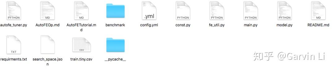
NNI treats AutoFeatureENG as a two-steps-task, feature generation exploration and feature selection. Feature generation exploration is mainly about feature derivation and high-order feature combination.
04 Feature Exploration
For feature derivation, NNI offers many operations which could automatically generate new features, which list as following :
count: Count encoding is based on replacing categories with their counts computed on the train set, also named frequency encoding.
target: Target encoding is based on encoding categorical variable values with the mean of target variable per value.
embedding: Regard features as sentences, generate vectors using Word2Vec.
crosscout: Count encoding on more than one-dimension, alike CTR (Click Through Rate).
aggregete: Decide the aggregation functions of the features, including min/max/mean/var.
nunique: Statistics of the number of unique features.
histsta: Statistics of feature buckets, like histogram statistics.
Search space could be defined in a JSON file: to define how specific features intersect, which two columns intersect and how features generate from corresponding columns.
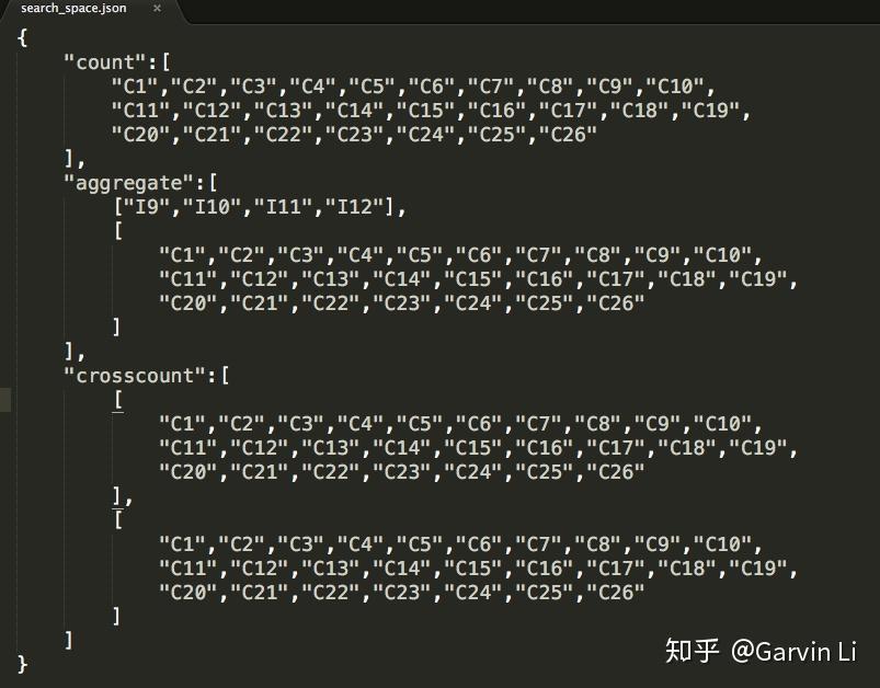
The picture shows us the procedure of defining search space. NNI provides count encoding for 1-order-op, as well as cross count encoding, aggerate statistics (min max var mean median nunique) for 2-order-op.
For example, we want to search the features which are a frequency encoding (valuecount) features on columns name {“C1”, …,” C26”}, in the following way:

we can define a cross frequency encoding (value count on cross dims) method on columns {“C1”,…,”C26”} x {“C1”,…,”C26”} in the following way:

The purpose of Exploration is to generate new features. You can use get_next_parameter function to get received feature candidates of one trial.
RECEIVED_PARAMS = nni.get_next_parameter()
05 Feature selection
To avoid feature explosion and overfitting, feature selection is necessary. In the feature selection of NNI-AutoFeatureENG, LightGBM (Light Gradient Boosting Machine), a gradient boosting framework developed by Microsoft, is mainly promoted.
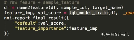
If you have used XGBoost or GBDT, you would know the algorithm based on tree structure can easily calculate the importance of each feature on results. LightGBM is able to make feature selection naturally.
The issue is that selected features might be applicable to GBDT (Gradient Boosting Decision Tree), but not to the linear algorithm like LR (Logistic Regression).
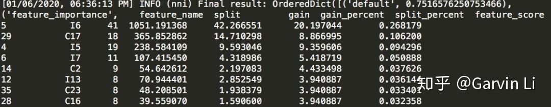
06 Summary
NNI’s AutoFeatureEng sets a well-established standard, showing us the operation procedure, available modules, which is highly convenient to use. However, a simple model is probably not enough for good results.
Suggestions to NNI
About Exploration: If consider using DNN (like xDeepFM) to extract high-order feature would be better.
About Selection: There could be more intelligent options, such as automatic selection system based on downstream models.
Conclusion: NNI could offer users some inspirations of design and it is a good open source project. I suggest researchers leverage it to accelerate the AI research.
Tips: Because the scripts of open source projects are compiled based on gcc7, Mac system may encounter problems of gcc (GNU Compiler Collection). The solution is as follows:
brew install libomp
Performance Measurement, Comparison and Analysis
Performance comparison and analysis can help users decide a proper algorithm (e.g., tuner, NAS algorithm) for their scenario. The following are some measurement and comparison data for users’ reference.
Neural Architecture Search Comparison
Posted by Anonymous Author
Train and Compare NAS (Neural Architecture Search) models including Autokeras, DARTS, ENAS and NAO.
Their source code link is as below:
Autokeras: https://github.com/jhfjhfj1/autokeras
Experiment Description
To avoid over-fitting in CIFAR-10, we also compare the models in the other five datasets including Fashion-MNIST, CIFAR-100, OUI-Adience-Age, ImageNet-10-1 (subset of ImageNet), ImageNet-10-2 (another subset of ImageNet). We just sample a subset with 10 different labels from ImageNet to make ImageNet-10-1 or ImageNet-10-2.
Dataset |
Training Size |
Numer of Classes |
Descriptions |
|---|---|---|---|
60,000 |
10 |
T-shirt/top, trouser, pullover, dress, coat, sandal, shirt, sneaker, bag and ankle boot. |
|
50,000 |
10 |
Airplanes, cars, birds, cats, deer, dogs, frogs, horses, ships and trucks. |
|
50,000 |
100 |
Similar to CIFAR-10 but with 100 classes and 600 images each. |
|
26,580 |
8 |
8 age groups/labels (0-2, 4-6, 8-13, 15-20, 25-32, 38-43, 48-53, 60-). |
|
9,750 |
10 |
Coffee mug, computer keyboard, dining table, wardrobe, lawn mower, microphone, swing, sewing machine, odometer and gas pump. |
|
9,750 |
10 |
Drum, banj, whistle, grand piano, violin, organ, acoustic guitar, trombone, flute and sax. |
We do not change the default fine-tuning technique in their source code. In order to match each task, the codes of input image shape and output numbers are changed.
Search phase time for all NAS methods is two days as well as the retrain time. Average results are reported based on three repeat times. Our evaluation machines have one Nvidia Tesla P100 GPU, 112GB of RAM and one 2.60GHz CPU (Intel E5-2690).
For NAO, it requires too much computing resources, so we only use NAO-WS which provides the pipeline script.
For AutoKeras, we used 0.2.18 version because it was the latest version when we started the experiment.
NAS Performance
NAS |
AutoKeras (%) |
ENAS (macro) (%) |
ENAS (micro) (%) |
DARTS (%) |
NAO-WS (%) |
|---|---|---|---|---|---|
Fashion-MNIST |
91.84 |
95.44 |
95.53 |
95.74 |
95.20 |
CIFAR-10 |
75.78 |
95.68 |
96.16 |
94.23 |
95.64 |
CIFAR-100 |
43.61 |
78.13 |
78.84 |
79.74 |
75.75 |
OUI-Adience-Age |
63.20 |
80.34 |
78.55 |
76.83 |
72.96 |
ImageNet-10-1 |
61.80 |
77.07 |
79.80 |
80.48 |
77.20 |
ImageNet-10-2 |
37.20 |
58.13 |
56.47 |
60.53 |
61.20 |
Unfortunately, we cannot reproduce all the results in the paper.
The best or average results reported in the paper:
NAS |
AutoKeras(%) |
ENAS (macro) (%) |
ENAS (micro) (%) |
DARTS (%) |
NAO-WS (%) |
|---|---|---|---|---|---|
CIFAR- 10 |
88.56(best) |
96.13(best) |
97.11(best) |
97.17(average) |
96.47(best) |
For AutoKeras, it has relatively worse performance across all datasets due to its random factor on network morphism.
For ENAS, ENAS (macro) shows good results in OUI-Adience-Age and ENAS (micro) shows good results in CIFAR-10.
For DARTS, it has a good performance on some datasets but we found its high variance in other datasets. The difference among three runs of benchmarks can be up to 5.37% in OUI-Adience-Age and 4.36% in ImageNet-10-1.
For NAO-WS, it shows good results in ImageNet-10-2 but it can perform very poorly in OUI-Adience-Age.
Reference
Jin, Haifeng, Qingquan Song, and Xia Hu. “Efficient neural architecture search with network morphism.” arXiv preprint arXiv:1806.10282 (2018).
Liu, Hanxiao, Karen Simonyan, and Yiming Yang. “Darts: Differentiable architecture search.” arXiv preprint arXiv:1806.09055 (2018).
Pham, Hieu, et al. “Efficient Neural Architecture Search via Parameters Sharing.” international conference on machine learning (2018): 4092-4101.
Luo, Renqian, et al. “Neural Architecture Optimization.” neural information processing systems (2018): 7827-7838.
Hyper Parameter Optimization Comparison
Posted by Anonymous Author
Comparison of Hyperparameter Optimization (HPO) algorithms on several problems.
Hyperparameter Optimization algorithms are list below:
All algorithms run in NNI local environment.
Machine Environment:
OS: Linux Ubuntu 16.04 LTS
CPU: Intel(R) Xeon(R) CPU E5-2690 v3 @ 2.60GHz 2600 MHz
Memory: 112 GB
NNI Version: v0.7
NNI Mode(local|pai|remote): local
Python version: 3.6
Is conda or virtualenv used?: Conda
is running in docker?: no
AutoGBDT Example
Nonconvex problem on the hyper-parameter search of AutoGBDT example.
{
"num_leaves": {
"_type": "choice",
"_value": [10, 12, 14, 16, 18, 20, 22, 24, 28, 32, 48, 64, 96, 128]
},
"learning_rate": {
"_type": "choice",
"_value": [0.00001, 0.0001, 0.001, 0.01, 0.05, 0.1, 0.2, 0.5]
},
"max_depth": {
"_type": "choice",
"_value": [-1, 2, 3, 4, 5, 6, 8, 10, 12, 14, 16, 18, 20, 22, 24, 28, 32, 48, 64, 96, 128]
},
"feature_fraction": {
"_type": "choice",
"_value": [0.9, 0.8, 0.7, 0.6, 0.5, 0.4, 0.3, 0.2]
},
"bagging_fraction": {
"_type": "choice",
"_value": [0.9, 0.8, 0.7, 0.6, 0.5, 0.4, 0.3, 0.2]
},
"bagging_freq": {
"_type": "choice",
"_value": [1, 2, 4, 8, 10, 12, 14, 16]
}
}
The total search space is 1,204,224, we set the number of maximum trial to 1000. The time limitation is 48 hours.
Algorithm |
Best loss |
Average of Best 5 Losses |
Average of Best 10 Losses |
|---|---|---|---|
Random Search |
0.418854 |
0.420352 |
0.421553 |
Random Search |
0.417364 |
0.420024 |
0.420997 |
Random Search |
0.417861 |
0.419744 |
0.420642 |
Grid Search |
0.498166 |
0.498166 |
0.498166 |
Evolution |
0.409887 |
0.409887 |
0.409887 |
Evolution |
0.413620 |
0.413875 |
0.414067 |
Evolution |
0.409887 |
0.409887 |
0.409887 |
Anneal |
0.414877 |
0.417289 |
0.418281 |
Anneal |
0.409887 |
0.409887 |
0.410118 |
Anneal |
0.413683 |
0.416949 |
0.417537 |
Metis |
0.416273 |
0.420411 |
0.422380 |
Metis |
0.420262 |
0.423175 |
0.424816 |
Metis |
0.421027 |
0.424172 |
0.425714 |
TPE |
0.414478 |
0.414478 |
0.414478 |
TPE |
0.415077 |
0.417986 |
0.418797 |
TPE |
0.415077 |
0.417009 |
0.418053 |
SMAC |
0.408386 |
0.408386 |
0.408386 |
SMAC |
0.414012 |
0.414012 |
0.414012 |
SMAC |
0.408386 |
0.408386 |
0.408386 |
BOHB |
0.410464 |
0.415319 |
0.417755 |
BOHB |
0.418995 |
0.420268 |
0.422604 |
BOHB |
0.415149 |
0.418072 |
0.418932 |
HyperBand |
0.414065 |
0.415222 |
0.417628 |
HyperBand |
0.416807 |
0.417549 |
0.418828 |
HyperBand |
0.415550 |
0.415977 |
0.417186 |
GP |
0.414353 |
0.418563 |
0.420263 |
GP |
0.414395 |
0.418006 |
0.420431 |
GP |
0.412943 |
0.416566 |
0.418443 |
In this example, all the algorithms are used with default parameters. For Metis, there are about 300 trials because it runs slowly due to its high time complexity O(n^3) in Gaussian Process.
RocksDB Benchmark ‘fillrandom’ and ‘readrandom’
DB_Bench is the main tool that is used to benchmark RocksDB‘s performance. It has so many hapermeter to tune.
The performance of DB_Bench is associated with the machine configuration and installation method. We run the DB_Benchin the Linux machine and install the Rock in shared library.
RocksDB: version 6.1
CPU: 6 * Intel(R) Xeon(R) CPU E5-2690 v4 @ 2.60GHz
CPUCache: 35840 KB
Keys: 16 bytes each
Values: 100 bytes each (50 bytes after compression)
Entries: 1000000
Latency: each IO request will take some time to complete, this is called the average latency. There are several factors that would affect this time including network connection quality and hard disk IO performance.
IOPS: IO operations per second, which means the amount of read or write operations that could be done in one seconds time.
IO size: the size of each IO request. Depending on the operating system and the application/service that needs disk access it will issue a request to read or write a certain amount of data at the same time.
Throughput (in MB/s) = Average IO size x IOPS
IOPS is related to online processing ability and we use the IOPS as the metric in my experiment.
{
"max_background_compactions": {
"_type": "quniform",
"_value": [1, 256, 1]
},
"block_size": {
"_type": "quniform",
"_value": [1, 500000, 1]
},
"write_buffer_size": {
"_type": "quniform",
"_value": [1, 130000000, 1]
},
"max_write_buffer_number": {
"_type": "quniform",
"_value": [1, 128, 1]
},
"min_write_buffer_number_to_merge": {
"_type": "quniform",
"_value": [1, 32, 1]
},
"level0_file_num_compaction_trigger": {
"_type": "quniform",
"_value": [1, 256, 1]
},
"level0_slowdown_writes_trigger": {
"_type": "quniform",
"_value": [1, 1024, 1]
},
"level0_stop_writes_trigger": {
"_type": "quniform",
"_value": [1, 1024, 1]
},
"cache_size": {
"_type": "quniform",
"_value": [1, 30000000, 1]
},
"compaction_readahead_size": {
"_type": "quniform",
"_value": [1, 30000000, 1]
},
"new_table_reader_for_compaction_inputs": {
"_type": "randint",
"_value": [1]
}
}
The search space is enormous (about 10^40) and we set the maximum number of trial to 100 to limit the computation resource.
Model |
Best IOPS (Repeat 1) |
Best IOPS (Repeat 2) |
Best IOPS (Repeat 3) |
|---|---|---|---|
Random |
449901 |
427620 |
477174 |
Anneal |
461896 |
467150 |
437528 |
Evolution |
436755 |
389956 |
389790 |
TPE |
378346 |
482316 |
468989 |
SMAC |
491067 |
490472 |
491136 |
Metis |
444920 |
457060 |
454438 |
Figure:

Model |
Best IOPS (Repeat 1) |
Best IOPS (Repeat 2) |
Best IOPS (Repeat 3) |
|---|---|---|---|
Random |
2276157 |
2285301 |
2275142 |
Anneal |
2286330 |
2282229 |
2284012 |
Evolution |
2286524 |
2283673 |
2283558 |
TPE |
2287366 |
2282865 |
2281891 |
SMAC |
2270874 |
2284904 |
2282266 |
Metis |
2287696 |
2283496 |
2277701 |
Figure:

Comparison of Filter Pruning Algorithms
To provide an initial insight into the performance of various filter pruning algorithms, we conduct extensive experiments with various pruning algorithms on some benchmark models and datasets. We present the experiment result in this document. In addition, we provide friendly instructions on the re-implementation of these experiments to facilitate further contributions to this effort.
Experiment Setting
The experiments are performed with the following pruners/datasets/models:
Models: VGG16, ResNet18, ResNet50
Datasets: CIFAR-10
Pruners:
These pruners are included:
Pruners with scheduling :
SimulatedAnnealing Pruner,NetAdapt Pruner,AutoCompress Pruner. Given the overal sparsity requirement, these pruners can automatically generate a sparsity distribution among different layers.One-shot pruners:
L1Filter Pruner,L2Filter Pruner,FPGM Pruner. The sparsity of each layer is set the same as the overall sparsity in this experiment.
Only filter pruning performances are compared here.
For the pruners with scheduling,
L1Filter Pruneris used as the base algorithm. That is to say, after the sparsities distribution is decided by the scheduling algorithm,L1Filter Pruneris used to performn real pruning.All the pruners listed above are implemented in nni.
Experiment Result
For each dataset/model/pruner combination, we prune the model to different levels by setting a series of target sparsities for the pruner.
Here we plot both Number of Weights - Performances curve and FLOPs - Performance curve. As a reference, we also plot the result declared in the paper AutoCompress: An Automatic DNN Structured Pruning Framework for Ultra-High Compression Rates for models VGG16 and ResNet18 on CIFAR-10.
The experiment result are shown in the following figures:
CIFAR-10, VGG16:

CIFAR-10, ResNet18:

CIFAR-10, ResNet50:

Analysis
From the experiment result, we get the following conclusions:
Given the constraint on the number of parameters, the pruners with scheduling (
AutoCompress Pruner,SimualatedAnnealing Pruner) performs better than the others when the constraint is strict. However, they have no such advantage in FLOPs/Performances comparison since only number of parameters constraint is considered in the optimization process;The basic algorithms
L1Filter Pruner,L2Filter Pruner,FPGM Prunerperforms very similarly in these experiments;NetAdapt Prunercan not achieve very high compression rate. This is caused by its mechanism that it prunes only one layer each pruning iteration. This leads to un-acceptable complexity if the sparsity per iteration is much lower than the overall sparisity constraint.
Experiments Reproduction
The experiment results are all collected with the default configuration of the pruners in nni, which means that when we call a pruner class in nni, we don’t change any default class arguments.
Both FLOPs and the number of parameters are counted with Model FLOPs/Parameters Counter after model speed up. This avoids potential issues of counting them of masked models.
The experiment code can be found here.
If you follow the practice in the example, for every single pruning experiment, the experiment result will be saved in JSON format as follows:
{ "performance": {"original": 0.9298, "pruned": 0.1, "speedup": 0.1, "finetuned": 0.7746}, "params": {"original": 14987722.0, "speedup": 167089.0}, "flops": {"original": 314018314.0, "speedup": 38589922.0} }
The experiment results are saved here. You can refer to analyze to plot new performance comparison figures.
Contribution
Pruners constrained by FLOPS/latency
More pruning algorithms/datasets/models
For algorithm implementation & experiment issues, please create an issue.
Use NNI on Google Colab
NNI can easily run on Google Colab platform. However, Colab doesn’t expose its public IP and ports, so by default you can not access NNI’s Web UI on Colab. To solve this, you need a reverse proxy software like ngrok or frp. This tutorial will show you how to use ngrok to access NNI’s Web UI on Colab.
How to Open NNI’s Web UI on Google Colab
Install required packages and softwares.
! pip install nni # install nni
! wget https://bin.equinox.io/c/4VmDzA7iaHb/ngrok-stable-linux-amd64.zip # download ngrok and unzip it
! unzip ngrok-stable-linux-amd64.zip
! mkdir -p nni_repo
! git clone https://github.com/microsoft/nni.git nni_repo/nni # clone NNI's offical repo to get examples
Register a ngrok account here, then connect to your account using your authtoken.
! ./ngrok authtoken <your-authtoken>
Start an NNI example on a port bigger than 1024, then start ngrok with the same port. If you want to use gpu, make sure gpuNum >= 1 in config.yml. Use
get_ipython()to start ngrok since it will be stuck if you use! ngrok http 5000 &.
! nnictl create --config nni_repo/nni/examples/trials/mnist-pytorch/config.yml --port 5000 &
get_ipython().system_raw('./ngrok http 5000 &')
Check the public url.
! curl -s http://localhost:4040/api/tunnels # don't change the port number 4040
You will see an url like http://xxxx.ngrok.io after step 4, open this url and you will find NNI’s Web UI. Have fun :)
Access Web UI with frp
frp is another reverse proxy software with similar functions. However, frp doesn’t provide free public urls, so you may need an server with public IP as a frp server. See here to know more about how to deploy frp.
External Repositories and References
With authors’ permission, we listed a set of NNI usage examples and relevant articles.
External Repositories
scikit-nni Hyper-parameter search for scikit-learn pipelines using NNI
Relevant Articles
Cost-effective Hyper-parameter Tuning using AdaptDL with NNI - Feb 23, 2021
(in Chinese) A summary of NNI new capabilities in NNI 2.0 - Jan 21, 2021
(in Chinese) A summary of NNI new capabilities in 2019 - Dec 26, 2019
Find thy hyper-parameters for scikit-learn pipelines using Microsoft NNI - Nov 6, 2019
(in Chinese) AutoML tools (Advisor, NNI and Google Vizier) comparison - Aug 05, 2019
Research and Publications
We are intensively working on both tool chain and research to make automatic model design and tuning really practical and powerful. On the one hand, our main work is tool chain oriented development. On the other hand, our research works aim to improve this tool chain, rethink challenging problems in AutoML (on both system and algorithm) and propose elegant solutions. Below we list some of our research works, we encourage more research works on this topic and encourage collaboration with us.
System Research
@inproceedings{zhang2020retiarii,
title={Retiarii: A Deep Learning Exploratory-Training Framework},
author={Zhang, Quanlu and Han, Zhenhua and Yang, Fan and Zhang, Yuge and Liu, Zhe and Yang, Mao and Zhou, Lidong},
booktitle={14th $\{$USENIX$\}$ Symposium on Operating Systems Design and Implementation ($\{$OSDI$\}$ 20)},
pages={919--936},
year={2020}
}
@inproceedings{liang2020autosys,
title={AutoSys: The Design and Operation of Learning-Augmented Systems},
author={Liang, Chieh-Jan Mike and Xue, Hui and Yang, Mao and Zhou, Lidong and Zhu, Lifei and Li, Zhao Lucis and Wang, Zibo and Chen, Qi and Zhang, Quanlu and Liu, Chuanjie and others},
booktitle={2020 $\{$USENIX$\}$ Annual Technical Conference ($\{$USENIX$\}$$\{$ATC$\}$ 20)},
pages={323--336},
year={2020}
}
@inproceedings{xiao2018gandiva,
title={Gandiva: Introspective cluster scheduling for deep learning},
author={Xiao, Wencong and Bhardwaj, Romil and Ramjee, Ramachandran and Sivathanu, Muthian and Kwatra, Nipun and Han, Zhenhua and Patel, Pratyush and Peng, Xuan and Zhao, Hanyu and Zhang, Quanlu and others},
booktitle={13th $\{$USENIX$\}$ Symposium on Operating Systems Design and Implementation ($\{$OSDI$\}$ 18)},
pages={595--610},
year={2018}
}
Algorithm Research
New Algorithms
@inproceedings{wang2020textnas,
title={TextNAS: A Neural Architecture Search Space Tailored for Text Representation.},
author={Wang, Yujing and Yang, Yaming and Chen, Yiren and Bai, Jing and Zhang, Ce and Su, Guinan and Kou, Xiaoyu and Tong, Yunhai and Yang, Mao and Zhou, Lidong},
booktitle={AAAI},
pages={9242--9249},
year={2020}
}
@article{peng2020cream,
title={Cream of the Crop: Distilling Prioritized Paths For One-Shot Neural Architecture Search},
author={Peng, Houwen and Du, Hao and Yu, Hongyuan and Li, Qi and Liao, Jing and Fu, Jianlong},
journal={Advances in Neural Information Processing Systems},
volume={33},
year={2020}
}
@inproceedings{li2018metis,
title={Metis: Robustly tuning tail latencies of cloud systems},
author={Li, Zhao Lucis and Liang, Chieh-Jan Mike and He, Wenjia and Zhu, Lianjie and Dai, Wenjun and Jiang, Jin and Sun, Guangzhong},
booktitle={2018 $\{$USENIX$\}$ Annual Technical Conference ($\{$USENIX$\}$$\{$ATC$\}$ 18)},
pages={981--992},
year={2018}
}
@article{Gao2021opevo,
title={OpEvo: An Evolutionary Method for Tensor Operator Optimization},
volume={35},
url={https://ojs.aaai.org/index.php/AAAI/article/view/17462},
number={14},
journal={Proceedings of the AAAI Conference on Artificial Intelligence},
author={Gao, Xiaotian and Cui, Wei and Zhang, Lintao and Yang, Mao},
year={2021}, month={May}, pages={12320-12327}
}
Measurement and Understanding
@article{zhang2020deeper,
title={Deeper insights into weight sharing in neural architecture search},
author={Zhang, Yuge and Lin, Zejun and Jiang, Junyang and Zhang, Quanlu and Wang, Yujing and Xue, Hui and Zhang, Chen and Yang, Yaming},
journal={arXiv preprint arXiv:2001.01431},
year={2020}
}
@article{zhang2020does,
title={How Does Supernet Help in Neural Architecture Search?},
author={Zhang, Yuge and Zhang, Quanlu and Yang, Yaming},
journal={arXiv preprint arXiv:2010.08219},
year={2020}
}
Applications
@inproceedings{chen2020autoadr,
title={AutoADR: Automatic Model Design for Ad Relevance},
author={Chen, Yiren and Yang, Yaming and Sun, Hong and Wang, Yujing and Xu, Yu and Shen, Wei and Zhou, Rong and Tong, Yunhai and Bai, Jing and Zhang, Ruofei},
booktitle={Proceedings of the 29th ACM International Conference on Information \& Knowledge Management},
pages={2365--2372},
year={2020}
}
FAQ
This page is for frequent asked questions and answers.
tmp folder fulled
nnictl will use tmp folder as a temporary folder to copy files under codeDir when executing experimentation creation. When met errors like below, try to clean up tmp folder first.
OSError: [Errno 28] No space left on device
Cannot get trials’ metrics in OpenPAI mode
In OpenPAI training mode, we start a rest server which listens on 51189 port in NNI Manager to receive metrcis reported from trials running in OpenPAI cluster. If you didn’t see any metrics from WebUI in OpenPAI mode, check your machine where NNI manager runs on to make sure 51189 port is turned on in the firewall rule.
Segmentation Fault (core dumped) when installing
make: *** [install-XXX] Segmentation fault (core dumped)
Please try the following solutions in turn:
Update or reinstall you current python’s pip like
python3 -m pip install -U pipInstall NNI with
--no-cache-dirflag likepython3 -m pip install nni --no-cache-dir
Job management error: getIPV4Address() failed because os.networkInterfaces().eth0 is undefined.
Your machine don’t have eth0 device, please set nniManagerIp in your config file manually.
Exceed the MaxDuration but didn’t stop
When the duration of experiment reaches the maximum duration, nniManager will not create new trials, but the existing trials will continue unless user manually stop the experiment.
Could not stop an experiment using nnictl stop
If you upgrade your NNI or you delete some config files of NNI when there is an experiment running, this kind of issue may happen because the loss of config file. You could use ps -ef | grep node to find the PID of your experiment, and use kill -9 {pid} to kill it manually.
Could not get default metric in webUI of virtual machines
Config the network mode to bridge mode or other mode that could make virtual machine’s host accessible from external machine, and make sure the port of virtual machine is not forbidden by firewall.
Could not open webUI link
Unable to open the WebUI may have the following reasons:
http://127.0.0.1,http://172.17.0.1andhttp://10.0.0.15are referred to localhost, if you start your experiment on the server or remote machine. You can replace the IP to your server IP to view the WebUI, likehttp://[your_server_ip]:8080If you still can’t see the WebUI after you use the server IP, you can check the proxy and the firewall of your machine. Or use the browser on the machine where you start your NNI experiment.
Another reason may be your experiment is failed and NNI may fail to get the experiment information. You can check the log of NNIManager in the following directory:
~/nni-experiments/[your_experiment_id]/log/nnimanager.log
Restful server start failed
Probably it’s a problem with your network config. Here is a checklist.
You might need to link
127.0.0.1withlocalhost. Add a line127.0.0.1 localhostto/etc/hosts.It’s also possible that you have set some proxy config. Check your environment for variables like
HTTP_PROXYorHTTPS_PROXYand unset if they are set.
NNI on Windows problems
Please refer to NNI on Windows
More FAQ issues
Help us improve
Please inquiry the problem in https://github.com/Microsoft/nni/issues to see whether there are other people already reported the problem, create a new one if there are no existing issues been created.
Contribute to NNI
Setup NNI development environment
NNI development environment supports Ubuntu 1604 (or above), and Windows 10 with Python3 64bit.
Installation
1. Clone source code
git clone https://github.com/Microsoft/nni.git
Note, if you want to contribute code back, it needs to fork your own NNI repo, and clone from there.
2. Install from source code
python3 -m pip install -U -r dependencies/setup.txt
python3 -m pip install -r dependencies/develop.txt
python3 setup.py develop
This installs NNI in development mode, so you don’t need to reinstall it after edit.
3. Check if the environment is ready
Now, you can try to start an experiment to check if your environment is ready. For example, run the command
nnictl create --config examples/trials/mnist-pytorch/config.yml
And open WebUI to check if everything is OK
4. Reload changes
Python
Nothing to do, the code is already linked to package folders.
TypeScript (Linux and macOS)
If
ts/nni_manageris changed, runyarn watchunder this folder. It will watch and build code continually. Thennictlneed to be restarted to reload NNI manager.If
ts/webuiis changed, runyarn dev, which will run a mock API server and a webpack dev server simultaneously. UseEXPERIMENTenvironment variable (e.g.,mnist-tfv1-running) to specify the mock data being used. Built-in mock experiments are listed insrc/webui/mock. An example of the full command isEXPERIMENT=mnist-tfv1-running yarn dev.
TypeScript (Windows)
Currently you must rebuild TypeScript modules with python3 setup.py build_ts after edit.
5. Submit Pull Request
All changes are merged to master branch from your forked repo. The description of Pull Request must be meaningful, and useful.
We will review the changes as soon as possible. Once it passes review, we will merge it to master branch.
For more contribution guidelines and coding styles, you can refer to the contributing document.
Contributing to Neural Network Intelligence (NNI)
Great!! We are always on the lookout for more contributors to our code base.
Firstly, if you are unsure or afraid of anything, just ask or submit the issue or pull request anyways. You won’t be yelled at for giving your best effort. The worst that can happen is that you’ll be politely asked to change something. We appreciate any sort of contributions and don’t want a wall of rules to get in the way of that.
However, for those individuals who want a bit more guidance on the best way to contribute to the project, read on. This document will cover all the points we’re looking for in your contributions, raising your chances of quickly merging or addressing your contributions.
Looking for a quickstart, get acquainted with our Get Started guide.
There are a few simple guidelines that you need to follow before providing your hacks.
Raising Issues
When raising issues, please specify the following:
Setup details needs to be filled as specified in the issue template clearly for the reviewer to check.
A scenario where the issue occurred (with details on how to reproduce it).
Errors and log messages that are displayed by the software.
Any other details that might be useful.
Submit Proposals for New Features
There is always something more that is required, to make it easier to suit your use-cases. Feel free to join the discussion on new features or raise a PR with your proposed change.
Fork the repository under your own github handle. After cloning the repository. Add, commit, push and sqaush (if necessary) the changes with detailed commit messages to your fork. From where you can proceed to making a pull request.
Contributing to Source Code and Bug Fixes
Provide PRs with appropriate tags for bug fixes or enhancements to the source code. Do follow the correct naming conventions and code styles when you work on and do try to implement all code reviews along the way.
If you are looking for How to develop and debug the NNI source code, you can refer to How to set up NNI developer environment doc file in the docs folder.
Similarly for Quick Start. For everything else, refer to NNI Home page.
Solve Existing Issues
Head over to issues to find issues where help is needed from contributors. You can find issues tagged with ‘good-first-issue’ or ‘help-wanted’ to contribute in.
A person looking to contribute can take up an issue by claiming it as a comment/assign their Github ID to it. In case there is no PR or update in progress for a week on the said issue, then the issue reopens for anyone to take up again. We need to consider high priority issues/regressions where response time must be a day or so.
Code Styles & Naming Conventions
We follow PEP8 for Python code and naming conventions, do try to adhere to the same when making a pull request or making a change. One can also take the help of linters such as
flake8orpylintWe also follow NumPy Docstring Style for Python Docstring Conventions. During the documentation building, we use sphinx.ext.napoleon to generate Python API documentation from Docstring.
For docstrings, please refer to numpydoc docstring guide and pandas docstring guide
For function docstring, description, Parameters, and Returns Yields are mandatory.
For class docstring, description, Attributes are mandatory.
For docstring to describe
dict, which is commonly used in our hyper-param format description, please refer to Internal Guideline on Writing Standards
Documentation
Our documentation is built with sphinx.
Before submitting the documentation change, please build homepage locally:
cd docs/en_US && make html, then you can see all the built documentation webpage under the folderdocs/en_US/_build/html. It’s also highly recommended taking care of every WARNING during the build, which is very likely the signal of a deadlink and other annoying issues.For links, please consider using relative paths first. However, if the documentation is written in reStructuredText format, and:
It’s an image link which needs to be formatted with embedded html grammar, please use global URL like
https://user-images.githubusercontent.com/44491713/51381727-e3d0f780-1b4f-11e9-96ab-d26b9198ba65.png, which can be automatically generated by dragging picture onto Github Issue Box.It cannot be re-formatted by sphinx, such as source code, please use its global URL. For source code that links to our github repo, please use URLs rooted at
https://github.com/Microsoft/nni/tree/master/(mnist.py for example).
Change Log
Release 2.5 - 11/2/2021
Model Compression
New major version of pruning framework (doc)
Iterative pruning is more automated, users can use less code to implement iterative pruning.
Support exporting intermediate models in the iterative pruning process.
The implementation of the pruning algorithm is closer to the paper.
Users can easily customize their own iterative pruning by using
PruningScheduler.Optimize the basic pruners underlying generate mask logic, easier to extend new functions.
Optimized the memory usage of the pruners.
MobileNetV2 end-to-end example (notebook)
Improved QAT quantizer (doc)
support dtype and scheme customization
support dp multi-gpu training
support load_calibration_config
Model speed-up now supports directly loading the mask (doc)
Support speed-up depth-wise convolution
Support bn-folding for LSQ quantizer
Support QAT and LSQ resume from PTQ
Added doc for observer quantizer (doc)
Neural Architecture Search
NAS benchmark (doc)
Support benchmark table lookup in experiments
New data preparation approach
Improved quick start doc
Experimental CGO execution engine (doc)
Hyper-Parameter Optimization
New training platform: Alibaba DSW+DLC (doc)
Support passing ConfigSpace definition directly to BOHB (doc) (thanks to khituras)
Reformatted experiment config doc
Added example config files for Windows (thanks to @politecat314)
FrameworkController now supports reuse mode
Fixed Bugs
Experiment cannot start due to platform timestamp format (issue #4077 #4083)
Cannot use
1e-5in search space (issue #4080)Dependency version conflict caused by ConfigSpace (issue #3909) (thanks to @jexxers)
Hardware-aware SPOS example does not work (issue #4198)
Web UI show wrong remaining time when duration exceeds limit (issue #4015)
cudnn.deterministic is always set in AMC pruner (#4117) thanks to @mstczuo
And…
New emoticons!

Release 2.4 - 8/11/2021
Major Updates
Neural Architecture Search
NAS visualization: visualize model graph through Netron (#3878)
Support NAS bench 101/201 on Retiarii framework (#3871 #3920)
Support hypermodule AutoActivation (#3868)
Support PyTorch v1.8/v1.9 (#3937)
Support Hardware-aware NAS with nn-Meter (#3938)
Enable fixed_arch on Retiarii (#3972)
Model Compression
Refactor of ModelSpeedup: auto shape/mask inference (#3462)
Added more examples for ModelSpeedup (#3880)
Support global sort for Taylor pruning (#3896)
Support TransformerHeadPruner (#3884)
Support batch normalization folding in QAT quantizer (#3911, thanks the external contributor @chenbohua3)
Support post-training observer quantizer (#3915, thanks the external contributor @chenbohua3)
Support ModelSpeedup for Slim Pruner (#4008)
Support TensorRT 8.0.0 in ModelSpeedup (#3866)
Hyper-parameter Tuning
Improve HPO benchmarks (#3925)
Improve type validation of user defined search space (#3975)
Training service & nnictl
Support JupyterLab (#3668 #3954)
Support viewing experiment from experiment folder (#3870)
Support kubeflow in training service reuse framework (#3919)
Support viewing trial log on WebUI for an experiment launched in view mode (#3872)
Minor Updates & Bug Fixes
Fix the failure of the exit of Retiarii experiment (#3899)
Fix exclude not supported in some config_list cases (#3815)
Fix bug in remote training service on reuse mode (#3941)
Improve IP address detection in modern way (#3860)
Fix bug of the search box on WebUI (#3935)
Fix bug in url_prefix of WebUI (#4051)
Support dict format of intermediate on WebUI (#3895)
Fix bug in openpai training service induced by experiment config v2 (#4027 #4057)
Improved doc (#3861 #3885 #3966 #4004 #3955)
Improved the API export_model in model compression (#3968)
Supported UnSqueeze in ModelSpeedup (#3960)
Thanks other external contributors: @Markus92 (#3936), @thomasschmied (#3963), @twmht (#3842)
Release 2.3 - 6/15/2021
Major Updates
Neural Architecture Search
Retiarii Framework (NNI NAS 2.0) Beta Release with new features:
Support new high-level APIs:
RepeatandCell(#3481)Support pure-python execution engine (#3605)
Support policy-based RL strategy (#3650)
Support nested ModuleList (#3652)
Improve documentation (#3785)
Note: there are more exciting features of Retiarii planned in the future releases, please refer to Retiarii Roadmap for more information.
Add new NAS algorithm: Blockwise DNAS FBNet (#3532, thanks the external contributor @alibaba-yiwuyao)
Model Compression
Support Auto Compression Framework (#3631)
Support slim pruner in Tensorflow (#3614)
Support LSQ quantizer (#3503, thanks the external contributor @chenbohua3)
Improve APIs for iterative pruners (#3507 #3688)
Training service & Rest
Support 3rd-party training service (#3662 #3726)
Support setting prefix URL (#3625 #3674 #3672 #3643)
Improve NNI manager logging (#3624)
Remove outdated TensorBoard code on nnictl (#3613)
Hyper-Parameter Optimization
Add new tuner: DNGO (#3479 #3707)
Add benchmark for tuners (#3644 #3720 #3689)
WebUI
Improve search parameters on trial detail page (#3651 #3723 #3715)
Make selected trials consistent after auto-refresh in detail table (#3597)
Add trial stdout button on local mode (#3653 #3690)
Examples & Documentation
Convert all trial examples’ from config v1 to config v2 (#3721 #3733 #3711 #3600)
Add new jupyter notebook examples (#3599 #3700)
Dev Excellent
Upgrade dependencies in Dockerfile (#3713 #3722)
Substitute PyYAML for
ruamel.yaml(#3702)Add pipelines for AML and hybrid training service and experiment config V2 (#3477 #3648)
Add pipeline badge in README (#3589)
Update issue bug report template (#3501)
Bug Fixes & Minor Updates
Fix syntax error on Windows (#3634)
Fix a logging related bug (#3705)
Fix a bug in GPU indices (#3721)
Fix a bug in FrameworkController (#3730)
Fix a bug in
export_data_url format(#3665)Report version check failure as a warning (#3654)
Fix bugs and lints in nnictl (#3712)
Fix bug of
optimize_modeon WebUI (#3731)Fix bug of
useActiveGpuin AML v2 config (#3655)Fix bug of
experiment_working_directoryin Retiarii config (#3607)Fix a bug in mask conflict (#3629, thanks the external contributor @Davidxswang)
Fix a bug in model speedup shape inference (#3588, thanks the external contributor @Davidxswang)
Fix a bug in multithread on Windows (#3604, thanks the external contributor @Ivanfangsc)
Delete redundant code in training service (#3526, thanks the external contributor @maxsuren)
Fix typo in DoReFa compression doc (#3693, thanks the external contributor @Erfandarzi)
Update docstring in model compression (#3647, thanks the external contributor @ichejun)
Fix a bug when using Kubernetes container (#3719, thanks the external contributor @rmfan)
Release 2.2 - 4/26/2021
Major updates
Neural Architecture Search
Improve NAS 2.0 (Retiarii) Framework (Alpha Release)
Support local debug mode (#3476)
Support nesting
ValueChoiceinLayerChoice(#3508)Support dict/list type in
ValueChoice(#3508)Improve the format of export architectures (#3464)
Refactor of NAS examples (#3513)
Refer to here for Retiarii Roadmap
Model Compression
Support speedup for mixed precision quantization model (Experimental) (#3488 #3512)
Support model export for quantization algorithm (#3458 #3473)
Support model export in model compression for TensorFlow (#3487)
Improve documentation (#3482)
nnictl & nni.experiment
Add native support for experiment config V2 (#3466 #3540 #3552)
Add resume and view mode in Python API
nni.experiment(#3490 #3524 #3545)
Training Service
Support umount for shared storage in remote training service (#3456)
Support Windows as the remote training service in reuse mode (#3500)
Remove duplicated env folder in remote training service (#3472)
Add log information for GPU metric collector (#3506)
Enable optional Pod Spec for FrameworkController platform (#3379, thanks the external contributor @mbu93)
WebUI
Support launching TensorBoard on WebUI (#3454 #3361 #3531)
Upgrade echarts-for-react to v5 (#3457)
Add wrap for dispatcher/nnimanager log monaco editor (#3461)
Bug Fixes
Fix bug of FLOPs counter (#3497)
Fix bug of hyper-parameter Add/Remove axes and table Add/Remove columns button conflict (#3491)
Fix bug that monaco editor search text is not displayed completely (#3492)
Fix bug of Cream NAS (#3498, thanks the external contributor @AliCloud-PAI)
Fix typos in docs (#3448, thanks the external contributor @OliverShang)
Fix typo in NAS 1.0 (#3538, thanks the external contributor @ankitaggarwal23)
Release 2.1 - 3/10/2021
Major updates
Neural architecture search
Improve NAS 2.0 (Retiarii) Framework (Improved Experimental)
Improve the robustness of graph generation and code generation for PyTorch models (#3365)
Support the inline mutation API
ValueChoice(#3349 #3382)Improve the design and implementation of Model Evaluator (#3359 #3404)
Support Random/Grid/Evolution exploration strategies (i.e., search algorithms) (#3377)
Refer to here for Retiarii Roadmap
Training service
Support shared storage for reuse mode (#3354)
Support Windows as the local training service in hybrid mode (#3353)
Remove PAIYarn training service (#3327)
Add “recently-idle” scheduling algorithm (#3375)
Deprecate
preCommandand enablepythonPathfor remote training service (#3284 #3410)Refactor reuse mode temp folder (#3374)
nnictl & nni.experiment
Migrate
nniclito new Python APInni.experiment(#3334)Refactor the way of specifying tuner in experiment Python API (
nni.experiment), more aligned withnnictl(#3419)
WebUI
Support showing the assigned training service of each trial in hybrid mode on WebUI (#3261 #3391)
Support multiple selection for filter status in experiments management page (#3351)
Improve overview page (#3316 #3317 #3352)
Support copy trial id in the table (#3378)
Documentation
Improve model compression examples and documentation (#3326 #3371)
Add Python API examples and documentation (#3396)
Add SECURITY doc (#3358)
Add ‘What’s NEW!’ section in README (#3395)
Update English contributing doc (#3398, thanks external contributor @Yongxuanzhang)
Bug fixes
Fix AML outputs path and python process not killed (#3321)
Fix bug that an experiment launched from Python cannot be resumed by nnictl (#3309)
Fix import path of network morphism example (#3333)
Fix bug in the tuple unpack (#3340)
Fix bug of security for arbitrary code execution (#3311, thanks external contributor @huntr-helper)
Fix
NoneTypeerror on jupyter notebook (#3337, thanks external contributor @tczhangzhi)Fix bugs in Retiarii (#3339 #3341 #3357, thanks external contributor @tczhangzhi)
Fix bug in AdaptDL mode example (#3381, thanks external contributor @ZeyaWang)
Fix the spelling mistake of assessor (#3416, thanks external contributor @ByronCHAO)
Fix bug in ruamel import (#3430, thanks external contributor @rushtehrani)
Release 2.0 - 1/14/2021
Major updates
Neural architecture search
Support an improved NAS framework: Retiarii (experimental)
Feature roadmap (issue #3301)
Documentation (#3221 #3282 #3287)
Support a new NAS algorithm: Cream (#2705)
Add a new NAS benchmark for NLP model search (#3140)
Training service
Support hybrid training service (#3097 #3251 #3252)
Support AdlTrainingService, a new training service based on Kubernetes (#3022, thanks external contributors Petuum @pw2393)
Model compression
Support pruning schedule for fpgm pruning algorithm (#3110)
ModelSpeedup improvement: support torch v1.7 (updated graph_utils.py) (#3076)
Improve model compression utility: model flops counter (#3048 #3265)
WebUI & nnictl
Support experiments management on WebUI, add a web page for it (#3081 #3127)
Improve the layout of overview page (#3046 #3123)
Add navigation bar on the right for logs and configs; add expanded icons for table (#3069 #3103)
Others
Support launching an experiment from Python code (#3111 #3210 #3263)
Refactor builtin/customized tuner installation (#3134)
Support new experiment configuration V2 (#3138 #3248 #3251)
Reorganize source code directory hierarchy (#2962 #2987 #3037)
Change SIGKILL to SIGTERM in local mode when cancelling trial jobs (#3173)
Refector hyperband (#3040)
Documentation
Port markdown docs to reStructuredText docs and introduce
githublink(#3107)List related research and publications in doc (#3150)
Add tutorial of saving and loading quantized model (#3192)
Remove paiYarn doc and add description of
reuseconfig in remote mode (#3253)Update EfficientNet doc to clarify repo versions (#3158, thanks external contributor @ahundt)
Bug fixes
Fix exp-duration pause timing under NO_MORE_TRIAL status (#3043)
Fix bug in NAS SPOS trainer, apply_fixed_architecture (#3051, thanks external contributor @HeekangPark)
Fix
_compute_hessianbug in NAS DARTS (PyTorch version) (#3058, thanks external contributor @hroken)Fix bug of conv1d in the cdarts utils (#3073, thanks external contributor @athaker)
Fix the handling of unknown trials when resuming an experiment (#3096)
Fix bug of kill command under Windows (#3106)
Fix lazy logging (#3108, thanks external contributor @HarshCasper)
Fix checkpoint load and save issue in QAT quantizer (#3124, thanks external contributor @eedalong)
Fix quant grad function calculation error (#3160, thanks external contributor @eedalong)
Fix device assignment bug in quantization algorithm (#3212, thanks external contributor @eedalong)
Fix bug in ModelSpeedup and enhance UT for it (#3279)
and others (#3063 #3065 #3098 #3109 #3125 #3143 #3156 #3168 #3175 #3180 #3181 #3183 #3203 #3205 #3207 #3214 #3216 #3219 #3223 #3224 #3230 #3237 #3239 #3240 #3245 #3247 #3255 #3257 #3258 #3262 #3263 #3267 #3269 #3271 #3279 #3283 #3289 #3290 #3295)
Release 1.9 - 10/22/2020
Major updates
Neural architecture search
Support regularized evolution algorithm for NAS scenario (#2802)
Add NASBench201 in search space zoo (#2766)
Model compression
AMC pruner improvement: support resnet, support reproduction of the experiments (default parameters in our example code) in AMC paper (#2876 #2906)
Support constraint-aware on some of our pruners to improve model compression efficiency (#2657)
Support “tf.keras.Sequential” in model compression for TensorFlow (#2887)
Support customized op in the model flops counter (#2795)
Support quantizing bias in QAT quantizer (#2914)
Training service
Support configuring python environment using “preCommand” in remote mode (#2875)
Support AML training service in Windows (#2882)
Support reuse mode for remote training service (#2923)
WebUI & nnictl
The “Overview” page on WebUI is redesigned with new layout (#2914)
Upgraded node, yarn and FabricUI, and enabled Eslint (#2894 #2873 #2744)
Add/Remove columns in hyper-parameter chart and trials table in “Trials detail” page (#2900)
JSON format utility beautify on WebUI (#2863)
Support nnictl command auto-completion (#2857)
UT & IT
Add integration test for experiment import and export (#2878)
Add integration test for user installed builtin tuner (#2859)
Add unit test for nnictl (#2912)
Documentation
Refactor of the document for model compression (#2919)
Bug fixes
Bug fix of naïve evolution tuner, correctly deal with trial fails (#2695)
Resolve the warning “WARNING (nni.protocol) IPC pipeline not exists, maybe you are importing tuner/assessor from trial code?” (#2864)
Fix search space issue in experiment save/load (#2886)
Fix bug in experiment import data (#2878)
Fix annotation in remote mode (python 3.8 ast update issue) (#2881)
Support boolean type for “choice” hyper-parameter when customizing trial configuration on WebUI (#3003)
Release 1.8 - 8/27/2020
Major updates
Training service
Access trial log directly on WebUI (local mode only) (#2718)
Add OpenPAI trial job detail link (#2703)
Support GPU scheduler in reusable environment (#2627) (#2769)
Add timeout for
web_channelintrial_runner(#2710)Show environment error message in AzureML mode (#2724)
Add more log information when copying data in OpenPAI mode (#2702)
WebUI, nnictl and nnicli
Improve hyper-parameter parallel coordinates plot (#2691) (#2759)
Add pagination for trial job list (#2738) (#2773)
Enable panel close when clicking overlay region (#2734)
Remove support for Multiphase on WebUI (#2760)
Support save and restore experiments (#2750)
Add intermediate results in export result (#2706)
Add command to list trial results with highest/lowest metrics (#2747)
Neural architecture search
Search space zoo: ENAS and DARTS (#2589)
API to query intermediate results in NAS benchmark (#2728)
Model compression
Support the List/Tuple Construct/Unpack operation for TorchModuleGraph (#2609)
Model speedup improvement: Add support of DenseNet and InceptionV3 (#2719)
Support the multiple successive tuple unpack operations (#2768)
Doc of comparing the performance of supported pruners (#2742)
New pruners: Sensitivity pruner (#2684) and AMC pruner (#2573) (#2786)
TensorFlow v2 support in model compression (#2755)
Backward incompatible changes
Update the default experiment folder from
$HOME/nni/experimentsto$HOME/nni-experiments. If you want to view the experiments created by previous NNI releases, you can move the experiments folders from$HOME/nni/experimentsto$HOME/nni-experimentsmanually. (#2686) (#2753)Dropped support for Python 3.5 and scikit-learn 0.20 (#2778) (#2777) (2783) (#2787) (#2788) (#2790)
Others
Upgrade TensorFlow version in Docker image (#2732) (#2735) (#2720)
Examples
Remove gpuNum in assessor examples (#2641)
Documentation
Improve customized tuner documentation (#2628)
Fix several typos and grammar mistakes in documentation (#2637 #2638, thanks @tomzx)
Improve AzureML training service documentation (#2631)
Improve CI of Chinese translation (#2654)
Improve OpenPAI training service documentation (#2685)
Improve documentation of community sharing (#2640)
Add tutorial of Colab support (#2700)
Improve documentation structure for model compression (#2676)
Bug fixes
Fix mkdir error in training service (#2673)
Fix bug when using chmod in remote training service (#2689)
Fix dependency issue by making
_graph_utilsimported inline (#2675)Fix mask issue in
SimulatedAnnealingPruner(#2736)Fix intermediate graph zooming issue (#2738)
Fix issue when dict is unordered when querying NAS benchmark (#2728)
Fix import issue for gradient selector dataloader iterator (#2690)
Fix support of adding tens of machines in remote training service (#2725)
Fix several styling issues in WebUI (#2762 #2737)
Fix support of unusual types in metrics including NaN and Infinity (#2782)
Fix nnictl experiment delete (#2791)
Release 1.7 - 7/8/2020
Major Features
Training Service
Support AML(Azure Machine Learning) platform as NNI training service.
OpenPAI job can be reusable. When a trial is completed, the OpenPAI job won’t stop, and wait next trial. refer to reuse flag in OpenPAI config.
Neural Architecture Search (NAS)
Model Compression
Improve Model Speedup: track more dependencies among layers and automatically resolve mask conflict, support the speedup of pruned resnet.
Added new pruners, including three auto model pruning algorithms: NetAdapt Pruner, SimulatedAnnealing Pruner, AutoCompress Pruner, and ADMM Pruner.
Added model sensitivity analysis tool to help users find the sensitivity of each layer to the pruning.
Update lottery ticket pruner to export winning ticket.
Examples
Automatically optimize tensor operators on NNI with a new customized tuner OpEvo.
Built-in tuners/assessors/advisors
WebUI
Support visualizing nested search space more friendly.
Show trial’s dict keys in hyper-parameter graph.
Enhancements to trial duration display.
Others
Provide utility function to merge parameters received from NNI
Support setting paiStorageConfigName in pai mode
Documentation
Improve documentation and examples for NAS benchmarks.
Homepage migration to readthedoc.
Bug Fixes
Fix bug for model graph with shared nn.Module
Fix nodejs OOM when
make buildFix NASUI bugs
Fix duration and intermediate results pictures update issue.
Fix minor WebUI table style issues.
Release 1.6 - 5/26/2020
Major Features
New Features and improvement
Improve IPC limitation to 100W
improve code storage upload logic among trials in non-local platform
support
__version__for SDK versionsupport windows dev intall
Web UI
Show trial error message
finalize homepage layout
Refactor overview’s best trials module
Remove multiphase from webui
add tooltip for trial concurrency in the overview page
Show top trials for hyper-parameter graph
HPO Updates
Improve PBT on failure handling and support experiment resume for PBT
NAS Updates
NAS support for TensorFlow 2.0 (preview) TF2.0 NAS examples
Use OrderedDict for LayerChoice
Prettify the format of export
Replace layer choice with selected module after applied fixed architecture
Model Compression Updates
Model compression PyTorch 1.4 support
Training Service Updates
update pai yaml merge logic
support windows as remote machine in remote mode Remote Mode
Bug Fix
fix dev install
SPOS example crash when the checkpoints do not have state_dict
Fix table sort issue when experiment had failed trial
Support multi python env (conda, pyenv etc)
Release 1.5 - 4/13/2020
New Features and Documentation
Hyper-Parameter Optimizing
New tuner: Population Based Training (PBT)
Trials can now report infinity and NaN as result
Neural Architecture Search
New NAS algorithm: TextNAS
ENAS and DARTS now support visualization through web UI.
Model Compression
New Pruner: GradientRankFilterPruner
Compressors will validate configuration by default
Refactor: Adding optimizer as an input argument of pruner, for easy support of DataParallel and more efficient iterative pruning. This is a broken change for the usage of iterative pruning algorithms.
Model compression examples are refactored and improved
Added documentation for implementing compressing algorithm
Training Service
Kubeflow now supports pytorchjob crd v1 (thanks external contributor @jiapinai)
Experimental DLTS support
Overall Documentation Improvement
Documentation is significantly improved on grammar, spelling, and wording (thanks external contributor @AHartNtkn)
Fixed Bugs
ENAS cannot have more than one LSTM layers (thanks external contributor @marsggbo)
NNI manager’s timers will never unsubscribe (thanks external contributor @guilhermehn)
NNI manager may exhaust head memory (thanks external contributor @Sundrops)
Batch tuner does not support customized trials (#2075)
Experiment cannot be killed if it failed on start (#2080)
Non-number type metrics break web UI (#2278)
A bug in lottery ticket pruner
Other minor glitches
Release 1.4 - 2/19/2020
Major Features
Neural Architecture Search
Support C-DARTS algorithm and add the example using it
Support a preliminary version of ProxylessNAS and the corresponding example
Add unit tests for the NAS framework
Model Compression
Support DataParallel for compressing models, and provide an example of using DataParallel
Support model speedup for compressed models, in Alpha version
Training Service
Support complete PAI configurations by allowing users to specify PAI config file path
Add example config yaml files for the new PAI mode (i.e., paiK8S)
Support deleting experiments using sshkey in remote mode (thanks external contributor @tyusr)
WebUI
WebUI refactor: adopt fabric framework
Others
Support running NNI experiment at foreground, i.e.,
--foregroundargument innnictl create/resume/viewSupport canceling the trials in UNKNOWN state
Support large search space whose size could be up to 50mb (thanks external contributor @Sundrops)
Documentation
Improve the index structure of NNI readthedocs
Improve documentation for NAS
Improve documentation for the new PAI mode
Add QuickStart guidance for NAS and model compression
Improve documentation for the supported EfficientNet
Bug Fixes
Correctly support NaN in metric data, JSON compliant
Fix the out-of-range bug of
randinttype in search spaceFix the bug of wrong tensor device when exporting onnx model in model compression
Fix incorrect handling of nnimanagerIP in the new PAI mode (i.e., paiK8S)
Release 1.3 - 12/30/2019
Major Features
Neural Architecture Search Algorithms Support
Single Path One Shot algorithm and the example using it
Model Compression Algorithms Support
Knowledge Distillation algorithm and the example using itExample
Pruners
Training Service
NFS Support for PAI
Instead of using HDFS as default storage, since OpenPAI v0.11, OpenPAI can have NFS or AzureBlob or other storage as default storage. In this release, NNI extended the support for this recent change made by OpenPAI, and could integrate with OpenPAI v0.11 or later version with various default storage.
Kubeflow update adoption
Adopted the Kubeflow 0.7’s new supports for tf-operator.
Engineering (code and build automation)
Enforced ESLint on static code analysis.
Small changes & Bug Fixes
Release 1.2 - 12/02/2019
Major Features
-
New feature engineering interface
Feature selection algorithms: Gradient feature selector & GBDT selector
Neural Architecture Search (NAS) on NNI
NAS in classic mode (each trial runs independently)
Model compression
New model pruning algorithms: lottery ticket pruning approach, L1Filter pruner, Slim pruner, FPGM pruner
New model quantization algorithms: QAT quantizer, DoReFa quantizer
Support the API for exporting compressed model.
Training Service
Support OpenPAI token authentication
Examples:
Engineering Improvements
For remote training service, trial jobs require no GPU are now scheduled with round-robin policy instead of random.
Pylint rules added to check pull requests, new pull requests need to comply with these pylint rules.
Web Portal & User Experience
Support user to add customized trial.
User can zoom out/in in detail graphs, except Hyper-parameter.
Documentation
Improved NNI API documentation with more API docstring.
Bug fix
Fix the table sort issue when failed trials haven’t metrics. -Issue #1773
Maintain selected status(Maximal/Minimal) when the page switched. -PR#1710
Make hyper-parameters graph’s default metric yAxis more accurate. -PR#1736
Fix GPU script permission issue. -Issue #1665
Release 1.1 - 10/23/2019
Major Features
New tuner: PPO Tuner
Tuners can now use dedicated GPU resource (see
gpuIndicesin tutorial for details)Web UI improvements
Trials detail page can now list hyperparameters of each trial, as well as their start and end time (via “add column”)
Viewing huge experiment is now less laggy
More examples
Model compression toolkit - Alpha release: We are glad to announce the alpha release for model compression toolkit on top of NNI, it’s still in the experiment phase which might evolve based on usage feedback. We’d like to invite you to use, feedback and even contribute
Fixed Bugs
Multiphase job hangs when search space exhuasted (issue #1204)
nnictlfails when log not available (issue #1548)
Release 1.0 - 9/2/2019
Major Features
Tuners and Assessors
Support Auto-Feature generator & selection -Issue#877 -PR #1387
Provide auto feature interface
Tuner based on beam search
Add a parallel algorithm to improve the performance of TPE with large concurrency. -PR #1052
Support multiphase for hyperband -PR #1257
Training Service
Support private docker registry -PR #755
Engineering Improvements
Python wrapper for rest api, support retrieve the values of the metrics in a programmatic way PR #1318
New python API : get_experiment_id(), get_trial_id() -PR #1353 -Issue #1331 & -Issue#1368
Optimized NAS Searchspace -PR #1393
Unify NAS search space with _type – “mutable_type”e
Update random search tuner
Set gpuNum as optional -Issue #1365
Remove outputDir and dataDir configuration in PAI mode -Issue #1342
When creating a trial in Kubeflow mode, codeDir will no longer be copied to logDir -Issue #1224
Web Portal & User Experience
Show the best metric curve during search progress in WebUI -Issue #1218
Show the current number of parameters list in multiphase experiment -Issue1210 -PR #1348
Add “Intermediate count” option in AddColumn. -Issue #1210
Support search parameters value in WebUI -Issue #1208
Enable automatic scaling of axes for metric value in default metric graph -Issue #1360
Add a detailed documentation link to the nnictl command in the command prompt -Issue #1260
UX improvement for showing Error log -Issue #1173
Documentation
Update the docs structure -Issue #1231
(deprecated) Multi phase document improvement -Issue #1233 -PR #1242
Add configuration example
WebUI description improvement -PR #1419
Bug fix
(Bug fix)Fix the broken links in 0.9 release -Issue #1236
(Bug fix)Script for auto-complete
(Bug fix)Fix pipeline issue that it only check exit code of last command in a script. -PR #1417
(Bug fix)quniform fors tuners -Issue #1377
(Bug fix)’quniform’ has different meaning beween GridSearch and other tuner. -Issue #1335
(Bug fix)”nnictl experiment list” give the status of a “RUNNING” experiment as “INITIALIZED” -PR #1388
(Bug fix)SMAC cannot be installed if nni is installed in dev mode -Issue #1376
(Bug fix)The filter button of the intermediate result cannot be clicked -Issue #1263
(Bug fix)API “/api/v1/nni/trial-jobs/xxx” doesn’t show a trial’s all parameters in multiphase experiment -Issue #1258
(Bug fix)Succeeded trial doesn’t have final result but webui show ×××(FINAL) -Issue #1207
(Bug fix)IT for nnictl stop -Issue #1298
(Bug fix)fix security warning
(Bug fix)Hyper-parameter page broken -Issue #1332
(Bug fix)Run flake8 tests to find Python syntax errors and undefined names -PR #1217
Release 0.9 - 7/1/2019
Major Features
General NAS programming interface
Add
enas-modeandoneshot-modefor NAS interface: PR #1201
(deprecated) Multiphase experiment supports
Added new training service support for multiphase experiment: PAI mode supports multiphase experiment since v0.9.
Added multiphase capability for the following builtin tuners:
TPE, Random Search, Anneal, Naïve Evolution, SMAC, Network Morphism, Metis Tuner.
Web Portal
Enable trial comparation in Web Portal. For details, refer to View trials status
Allow users to adjust rendering interval of Web Portal. For details, refer to View Summary Page
show intermediate results more friendly. For details, refer to View trials status
-
nnictl experiment delete: delete one or all experiments, it includes log, result, environment information and cache. It uses to delete useless experiment result, or save disk space.nnictl platform clean: It uses to clean up disk on a target platform. The provided YAML file includes the information of target platform, and it follows the same schema as the NNI configuration file.
Bug fix and other changes
Tuner Installation Improvements: add sklearn to nni dependencies.
(Bug Fix) Failed to connect to PAI http code - Issue #1076
(Bug Fix) Validate file name for PAI platform - Issue #1164
(Bug Fix) Update GMM evaluation in Metis Tuner
(Bug Fix) Negative time number rendering in Web Portal - Issue #1182, Issue #1185
(Bug Fix) Hyper-parameter not shown correctly in WebUI when there is only one hyper parameter - Issue #1192
Release 0.8 - 6/4/2019
Major Features
Support NNI on Windows for OpenPAI/Remote mode
NNI running on windows for remote mode
NNI running on windows for OpenPAI mode
Advanced features for using GPU
Run multiple trial jobs on the same GPU for local and remote mode
Run trial jobs on the GPU running non-NNI jobs
Kubeflow v1beta2 operator
Support Kubeflow TFJob/PyTorchJob v1beta2
General NAS programming interface
Provide NAS programming interface for users to easily express their neural architecture search space through NNI annotation
Provide a new command
nnictl trial codegenfor debugging the NAS codeTutorial of NAS programming interface, example of NAS on MNIST, customized random tuner for NAS
Support resume tuner/advisor’s state for experiment resume
For experiment resume, tuner/advisor will be resumed by replaying finished trial data
Web Portal
Improve the design of copying trial’s parameters
Support ‘randint’ type in hyper-parameter graph
Use should ComponentUpdate to avoid unnecessary render
Bug fix and other changes
Bug fix that
nnictl updatehas inconsistent command stylesSupport import data for SMAC tuner
Bug fix that experiment state transition from ERROR back to RUNNING
Fix bug of table entries
Nested search space refinement
Refine ‘randint’ type and support lower bound
Release 0.7 - 4/29/2018
Major Features
-
NNI running on windows for local mode
-
Support a new advisor BOHB, which is a robust and efficient hyperparameter tuning algorithm, combines the advantages of Bayesian optimization and Hyperband
Support import and export experiment data through nnictl
Generate analysis results report after the experiment execution
Support import data to tuner and advisor for tuning
Designated gpu devices for NNI trial jobs
Specify GPU devices for NNI trial jobs by gpuIndices configuration, if gpuIndices is set in experiment configuration file, only the specified GPU devices are used for NNI trial jobs.
Web Portal enhancement
Decimal format of metrics other than default on the Web UI
Hints in WebUI about Multi-phase
Enable copy/paste for hyperparameters as python dict
Enable early stopped trials data for tuners.
NNICTL provide better error message
nnictl provide more meaningful error message for YAML file format error
Bug fix
Unable to kill all python threads after nnictl stop in async dispatcher mode
nnictl –version does not work with make dev-install
All trail jobs status stays on ‘waiting’ for long time on OpenPAI platform
Release 0.6 - 4/2/2019
Major Features
-
check whether the version is consistent between nniManager and trialKeeper
Report final metrics for early stop job
If includeIntermediateResults is true, the last intermediate result of the trial that is early stopped by assessor is sent to tuner as final result. The default value of includeIntermediateResults is false.
-
Adds two pipes to separate message receiving channels for tuner and assessor.
Make log collection feature configurable
Add intermediate result graph for all trials
Bug fix
Fix the bug that doesn’t show any result if metrics is dict
Fix the number calculation issue for float types in hyperband
Fix a bug in the search space conversion in SMAC tuner
Fix the WebUI issue when parsing experiment.json with illegal format
Fix cold start issue in Metis Tuner
Release 0.5.2 - 3/4/2019
Improvements
Curve fitting assessor performance improvement.
Documentation
Chinese version document: https://nni.readthedocs.io/zh/latest/
Debuggability/serviceability document: https://nni.readthedocs.io/en/latest/Tutorial/HowToDebug.html
Tuner assessor reference: https://nni.readthedocs.io/en/latest/sdk_reference.html
Bug Fixes and Other Changes
Fix a race condition bug that does not store trial job cancel status correctly.
Fix search space parsing error when using SMAC tuner.
Fix cifar10 example broken pipe issue.
Add unit test cases for nnimanager and local training service.
Add integration test azure pipelines for remote machine, OpenPAI and kubeflow training services.
Support Pylon in OpenPAI webhdfs client.
Release 0.5.1 - 1/31/2018
Improvements
Making log directory configurable
Support different levels of logs, making it easier for debugging
Documentation
Reorganized documentation & New Homepage Released: https://nni.readthedocs.io/en/latest/
Bug Fixes and Other Changes
Fix the bug of installation in python virtualenv, and refactor the installation logic
Fix the bug of HDFS access failure on OpenPAI mode after OpenPAI is upgraded.
Fix the bug that sometimes in-place flushed stdout makes experiment crash
Release 0.5.0 - 01/14/2019
Major Features
New tuner and assessor supports
Support Metis tuner as a new NNI tuner. Metis algorithm has been proofed to be well performed for online hyper-parameter tuning.
Support ENAS customized tuner, a tuner contributed by github community user, is an algorithm for neural network search, it could learn neural network architecture via reinforcement learning and serve a better performance than NAS.
Support Curve fitting assessor for early stop policy using learning curve extrapolation.
Advanced Support of Weight Sharing: Enable weight sharing for NAS tuners, currently through NFS.
Training Service Enhancement
FrameworkController Training service: Support run experiments using frameworkcontroller on kubernetes
FrameworkController is a Controller on kubernetes that is general enough to run (distributed) jobs with various machine learning frameworks, such as tensorflow, pytorch, MXNet.
NNI provides unified and simple specification for job definition.
MNIST example for how to use FrameworkController.
User Experience improvements
A better trial logging support for NNI experiments in OpenPAI, Kubeflow and FrameworkController mode:
An improved logging architecture to send stdout/stderr of trials to NNI manager via Http post. NNI manager will store trial’s stdout/stderr messages in local log file.
Show the link for trial log file on WebUI.
Support to show final result’s all key-value pairs.
Release 0.4.1 - 12/14/2018
Major Features
New tuner supports
Support network morphism as a new tuner
Training Service improvements
Migrate Kubeflow training service‘s dependency from kubectl CLI to Kubernetes API client
Pytorch-operator support for Kubeflow training service
Improvement on local code files uploading to OpenPAI HDFS
Fixed OpenPAI integration WebUI bug: WebUI doesn’t show latest trial job status, which is caused by OpenPAI token expiration
NNICTL improvements
Show version information both in nnictl and WebUI. You can run nnictl -v to show your current installed NNI version
WebUI improvements
Enable modify concurrency number during experiment
Add feedback link to NNI github ‘create issue’ page
Enable customize top 10 trials regarding to metric numbers (largest or smallest)
Enable download logs for dispatcher & nnimanager
Enable automatic scaling of axes for metric number
Update annotation to support displaying real choice in searchspace
New examples
FashionMnist, work together with network morphism tuner
Distributed MNIST example written in PyTorch
Release 0.4 - 12/6/2018
Major Features
-
Support tf-operator
Distributed trial example on Kubeflow
Support launch NNI experiment on MAC
WebUI
UI support for hyperband tuner
Remove tensorboard button
Show experiment error message
Show line numbers in search space and trial profile
Support search a specific trial by trial number
Show trial’s hdfsLogPath
Download experiment parameters
Others
Asynchronous dispatcher
Docker file update, add pytorch library
Refactor ‘nnictl stop’ process, send SIGTERM to nni manager process, rather than calling stop Rest API.
OpenPAI training service bug fix
Support NNI Manager IP configuration(nniManagerIp) in OpenPAI cluster config file, to fix the issue that user’s machine has no eth0 device
File number in codeDir is capped to 1000 now, to avoid user mistakenly fill root dir for codeDir
Don’t print useless ‘metrics is empty’ log in OpenPAI job’s stdout. Only print useful message once new metrics are recorded, to reduce confusion when user checks OpenPAI trial’s output for debugging purpose
Add timestamp at the beginning of each log entry in trial keeper.
Release 0.3.0 - 11/2/2018
NNICTL new features and updates
Support running multiple experiments simultaneously.
Before v0.3, NNI only supports running single experiment once a time. After this release, users are able to run multiple experiments simultaneously. Each experiment will require a unique port, the 1st experiment will be set to the default port as previous versions. You can specify a unique port for the rest experiments as below:
nnictl create --port 8081 --config <config file path>Support updating max trial number. use
nnictl update --helpto learn more. Or refer to NNICTL Spec for the fully usage of NNICTL.
API new features and updates
**breaking change**: nn.get_parameters() is refactored to nni.get_next_parameter. All examples of prior releases can not run on v0.3, please clone nni repo to get new examples. If you had applied NNI to your own codes, please update the API accordingly.
New API nni.get_sequence_id(). Each trial job is allocated a unique sequence number, which can be retrieved by nni.get_sequence_id() API.
git clone -b v0.3 https://github.com/microsoft/nni.git
nni.report_final_result(result) API supports more data types for result parameter.
It can be of following types:
int
float
A python dict containing ‘default’ key, the value of ‘default’ key should be of type int or float. The dict can contain any other key value pairs.
New tuner support
Batch Tuner which iterates all parameter combination, can be used to submit batch trial jobs.
New examples
A NNI Docker image for public usage:
docker pull msranni/nni:latest
New trial example: NNI Sklearn Example
New competition example: Kaggle Competition TGS Salt Example
Others
UI refactoring, refer to WebUI doc for how to work with the new UI.
Continuous Integration: NNI had switched to Azure pipelines
Release 0.2.0 - 9/29/2018
Major Features
Support OpenPAI Training Platform (See here for instructions about how to submit NNI job in pai mode)
Support training services on pai mode. NNI trials will be scheduled to run on OpenPAI cluster
NNI trial’s output (including logs and model file) will be copied to OpenPAI HDFS for further debugging and checking
Support SMAC tuner (See here for instructions about how to use SMAC tuner)
Support NNI installation on conda and python virtual environment
Others
Update ga squad example and related documentation
WebUI UX small enhancement and bug fix
Release 0.1.0 - 9/10/2018 (initial release)
Initial release of Neural Network Intelligence (NNI).
Major Features
Installation and Deployment
Support pip install and source codes install
Support training services on local mode(including Multi-GPU mode) as well as multi-machines mode
Tuners, Assessors and Trial
Support AutoML algorithms including: hyperopt_tpe, hyperopt_annealing, hyperopt_random, and evolution_tuner
Support assessor(early stop) algorithms including: medianstop algorithm
Provide Python API for user defined tuners and assessors
Provide Python API for user to wrap trial code as NNI deployable codes
Experiments
Provide a command line toolkit ‘nnictl’ for experiments management
Provide a WebUI for viewing experiments details and managing experiments
Continuous Integration
Support CI by providing out-of-box integration with travis-ci on ubuntu
Others
Support simple GPU job scheduling